Introduction
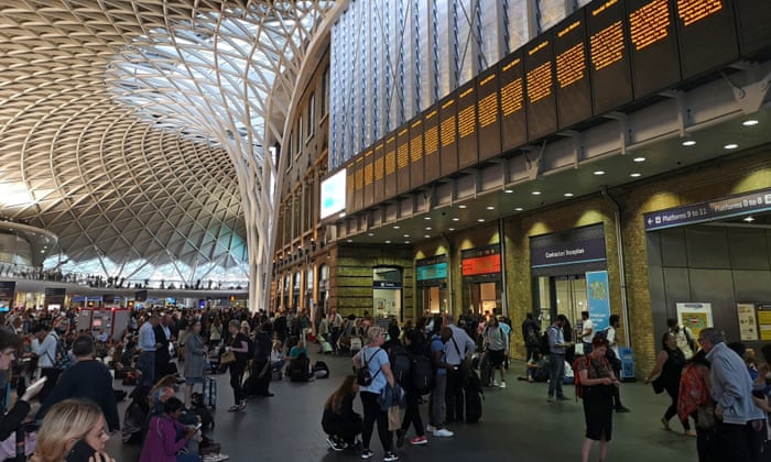
On Friday 9th August 2019, Britain suffered one of the worst power outages in recent years. Over 1 million people in England and Wales were cut off from power for nearly 9 hours, preventing numerous rail services from running during the rush hour.
Was this a statistical misfortune, or a systemic failure which caused the recent power outages?
Getting the data
To obtain the information required to do analysis of the events leading up to the catastrophic power outage, we will we will use a fantastic website, GridWatch Templar, which has realtime data as to the different power supplies, resources and frequencies. From the download page, I downloaded all the data from 27th May 2011 to the current time. Be patient; it will take a considerable amount of time to download the entire dataset (and as it is too large, I have not attached this csv file to this page). Also, as we will be carrying out analysis on such a large dataset, some cells will take a considerable amount of time to run.
Analysis of the frequencies
First, we import the dataset:
In[1]: data = Import["D:\\Programming\\GridWatch\\gridwatch.csv"];
The data which it contains:
In[2]: data[[1]]

Out[2]: {"id", "timestamp", "demand", "frequency", "coal", "nuclear", "ccgt", \
"wind", "pumped", "hydro", "biomass", "oil", "solar", "ocgt", \
"french_ict", "dutch_ict", "irish_ict", "ew_ict", "nemo", "other", \
"north_south", "scotland_england"}
To look at the frequencies:
In[3]: frequencies =
 If[#[[4]] == 0, Nothing, {DateObject[#[[2]]], #[[4]]}] & /@
  data[[2 ;;]];
To show the minimum value:
In[4]: MinimalBy[frequencies, Last]

Out[4]: {{DateObject[{2019, 8, 9, 15, 55, 37}, "Instant", "Gregorian", 1.],
  48.889}}

In[5]: DateListPlot[frequencies, PlotRange -> All, AxesLabel -> {"Time", "Hz"}]
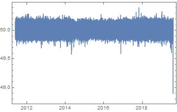
This is not particularly enlightening; although it does show how dramatic the recent drop of frequency is. In fact, it is known that if the frequency drops below 49.5 Hz, a blackout will occur - and this is the first time it has happened (at least since 2011).
Let's dive deeper - we'll use a normal distribution in approximation to the distribution:
In[6]: distribution = NormalDistribution[Mean[Last /@ frequencies], StandardDeviation[Last /@ frequencies]]

Out[6]: NormalDistribution[50.0012, 0.0584802]
Now plotting it gives:
In[7]: Show[Histogram[Last /@ newfreqs, Automatic, "ProbabilityDensity"],
 Plot[PDF[distribution, x], {x, 49.7, 50.3},
  PlotStyle -> Thick]]
This returns: 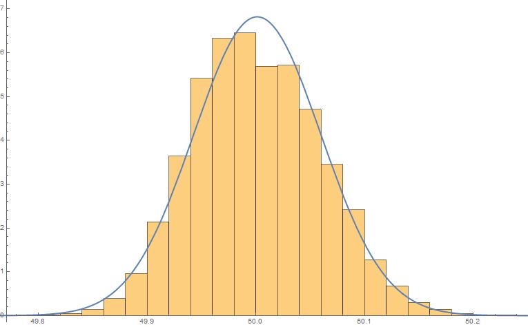
Observe how quickly this tapers off. Assuming the frequencies follow that normal distribution, the probability of this occurring is:
In[8]: Probability[freq <= 49.5, freq \[Distributed] distribution]

Out[8]: 5.1191*10^-18
So we can be very confident that this was not just a statistical mishap - there was a genuine, systemic cause for this event to occur (see the comment below for explanation of this).
Now let's take a closer look at what happened that day.
Focusing in further
A National Grid spokesperson said:
The root cause of yesterdays issue was not with our system but was a rare and unusual event, the almost simultaneous loss of two large generators, one gas and one offshore wind, at 4.54pm. We are still working with the generators to understand what caused the generation to be lost.
(courtesy of the the Guardian for this report). We will verify this report below.
First, we will zoom in on the interval between one day before and one day after the event occurred.
In[9]: timeinterval = Select[data[[2;;]],
 DateObject[{2019, 8, 9, 15, 55, 37}, "Instant", "Gregorian", 1.`] -
    Quantity[1, "Days"] <= DateObject[#[[2]]] <=
   DateObject[{2019, 8, 9, 15, 55, 37}, "Instant", "Gregorian", 1.`] +
     Quantity[1, "Days"] &]
(This specific time interval data is attached to this post).
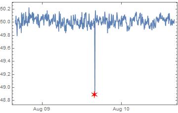
To visualise it the frequencies:
In[11]: timeintervalfreqs = {DateObject[#[[2]]], #[[4]]} & /@ timeinterval;

In[12]: DateListPlot[Out[51], PlotRange -> All,
 Epilog -> {Red,
   Text[Style["\[SixPointedStar]",
       20], #] & /@ {{DateObject[{2019, 8, 9, 15, 55, 37}, "Instant",
       "Gregorian", 1.`], 48.889`}}}]
which shows:
Now let's look at the specific types of energy generation:
In[13]: DateListPlot[
 Table[{DateObject[#[[2]]], #[[k]]} & /@ timeinterval, {k, 5, 21}],
 PlotLegends -> data[[1]][[5 ;;]], PlotRange -> All]
which returns 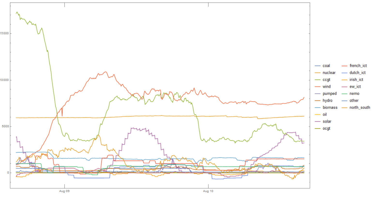
Now let's reduce down to the two energy sources which were mentioned in the report: namely, gas (or CCGT, OCGT), and offshore wind.
In[14]: indices = {3, 7, 8, 14};
DateListPlot[
 Table[{DateObject[#[[2]]], #[[k]]} & /@ timeinterval, {k, indices}],
 PlotLegends -> data[[1]][[indices]], PlotRange -> All,
 Epilog -> {Directive[{Thick, Red, Dashed}],
   Line[{{DateObject[{2019, 8, 9, 15, 55, 37}, "Instant", "Gregorian",
        1.`], 0}, {DateObject[{2019, 8, 9, 15, 55, 37}, "Instant",
       "Gregorian", 1.`], 40000}}]}]
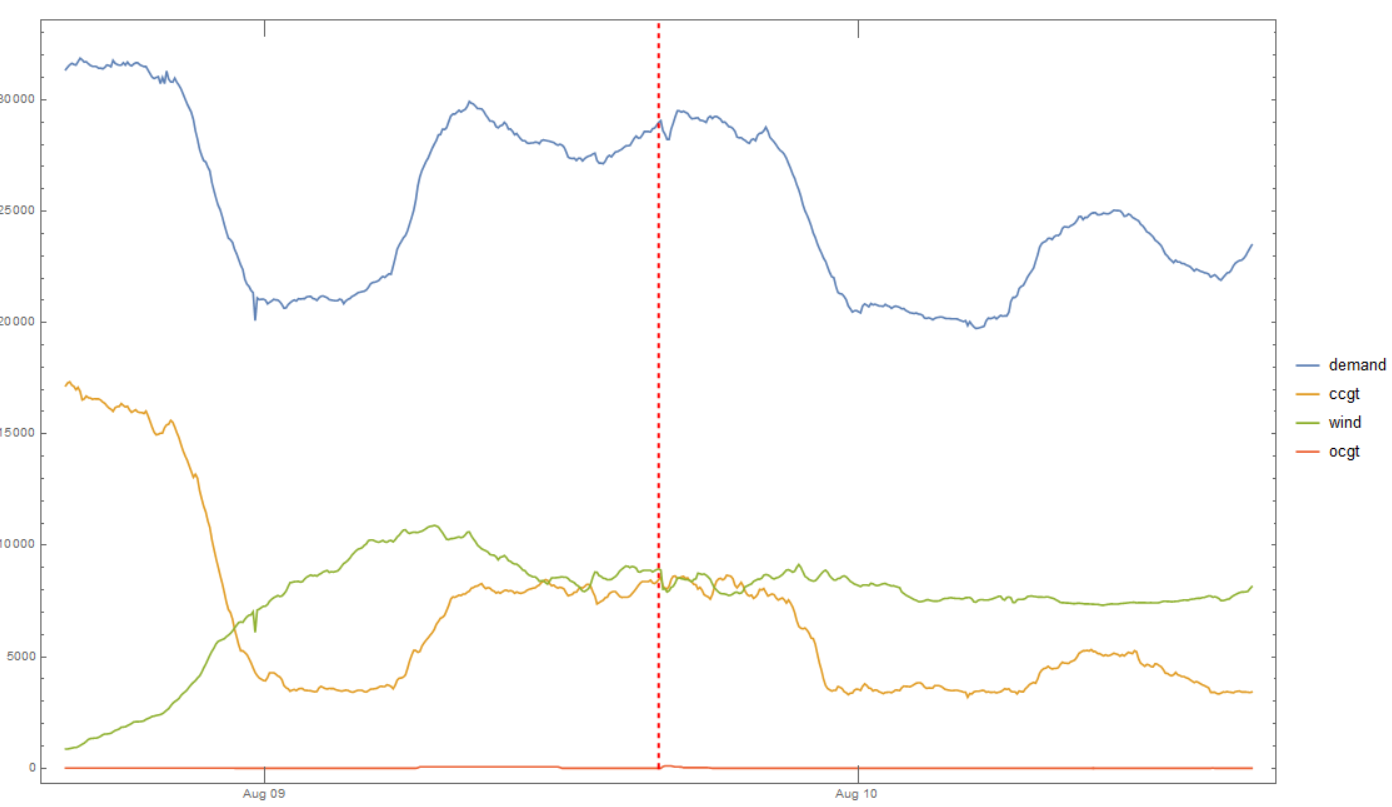
This clearly shows a drop in CCGT and wind power (and also the demand) subsequent to the incident.
Finding peaks for the CCGT data to find when the drop occurs:
In[15]: ccgtdata = {AbsoluteTime[#[[2]]], -#[[8]]} & /@ timeinterval;

In[16]: inter = Interpolation[ccgtdata[[All, 1]]];

In[17]: peaks = FindPeaks[ccgtdata[[All, 2]]];

In[18]: peak = Select[{inter[#1], #2} & @@@
  peaks, #[[1]] >=
   AbsoluteTime[
    DateObject[{2019, 8, 9, 15, 55, 37}, "Instant", "Gregorian",
     1.`]] &][[1, 1]] (*This calculates the first trough since the event took place*)

Out[18]: 3774356135
This means that, 20 minutes after the frequency collapses, the CCGT (and the Wind power) supply decrease dramatically.
Conclusion
At 3:55 PM GMT +1 (so really 4:55 PM, confirming the report - this is on account of BST) on Friday the 9th of August, for the first time since 2011 (and probably many years before), frequency reached levels below 49.5 Hz, at which point blackouts would take place, affecting nearly 1 million people and disrupting multiple rail services across England and Wales. According to the National Grid, this had almost happened 3 times before this one took place; our data can confirm this (see the graph below input 5). We can be certain that this was not a statistical oddity; in fact, around 20 minutes later, we begin to see that the CCGT and offshore wind supplies decrease, which confirms the report stating that both had cut out simultaneously. Hopefully this will never happen again. With this dataset at hand, it seems likely that these outages could be more foreseen in the future.
 Attachments:


