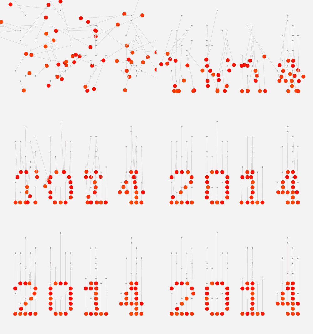
I guess it is typical for Russian greetings to come with necessity to brush up on your theoretical mechanics. As you can see below there are 61 randomly constructed friction-damped pendulums swinging in chaos just to eventually converge to cheerful red 2014 which is inscribed in their stable equilibrium positions.
Watch them here dancing under inspirational classical music.
Our
sister Russian community counts almost 2000 members from all around Eastern Europe and beyond. Over the holidays they have enjoyed this Wolfram Language artwork designed by
Roman Osipov and wish to share it with us. Original notebook in Russian can be
dowloaded here. So let me translate the inner workings.

Take a simple string with some simple formatting:
string = Style["2014", FontFamily -> "Arial", 11];
Let's Rasterize, Binarize and Rotate the resulting image to the right by 90 degrees (necessary for to adjust for different coordinate systems in images and WL arrays):
image = ImageRotate[Binarize@Rasterize[string], -90 Degree];
Convert the image to a set of numbers corresponding to the two color values??, because it was binarized (1 - white, 0 - black):
imageData = ImageData[image];
Translate the image into a set of points, taking the indices of black pixels in Cartesian coordinates:
points = N[Position[imageData, 0]];
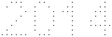
Look at the resulting set of points:
Graphics[Point[points], ImageSize -> 500]

Find how many points there are in the image:
lengthP = Length[points]
(* Out[] = 61 *)
We will now define a function, which solves the differential equation describing the pendulum with damping:
sol[x0_: 1, v0_: 0, s_: 1] := sol[x0, v0, s] =
NDSolve[{x''[t] + s x'[t] + 9.8 Sin[x[t]] == 0, x[0] == x0, x'[0] == v0}, x, {t, 0, 40}]
Here are some auxiliary functions that convert the differential equation obtained above into coordinates of the pendulum:
coord[t_, x0_: 1, v0_: 0, s_: 1] := coord[t, x0, v0, s] = x[t] /. sol[x0, v0, s][[1]];
rC[t_, {a_: 0, b_: 0}, R_: 1, x0_, v0_, s_] :=
rC[t, {a, b}, R, x0, v0, s] = {a, b} + R {Cos[coord[t, x0, v0, s] - Pi/2], Sin[coord[t, x0, v0, s] - Pi/2] + 1};
We now construct a function that transforms each of the points in a row in 2014, to a pendulum, which runs from a random position, with random initial velocity and suspended on a string of random length and has a random color:
color := Hue[RandomReal[{0, 1/5}]];
graphicsData[t_] =
Table[{R, x0, v0, s} = {RandomInteger[{1, 10}],
RandomReal[{-Pi, Pi}], RandomReal[{0, 1}], RandomReal[{0.2, 1}]};
currentCoords = rC[t, points[[n]], R, x0, v0, s];
{{LightGray, Thick, Line[{currentCoords, points[[n]] + {0, R}}]},
{AbsolutePointSize[6], Gray, Point[points[[n]] + {0, R}], White,
AbsolutePointSize[3], Point[points[[n]] + {0, R}]},
AbsolutePointSize[15], color, Point[currentCoords]},
{n, 1, lengthP}];
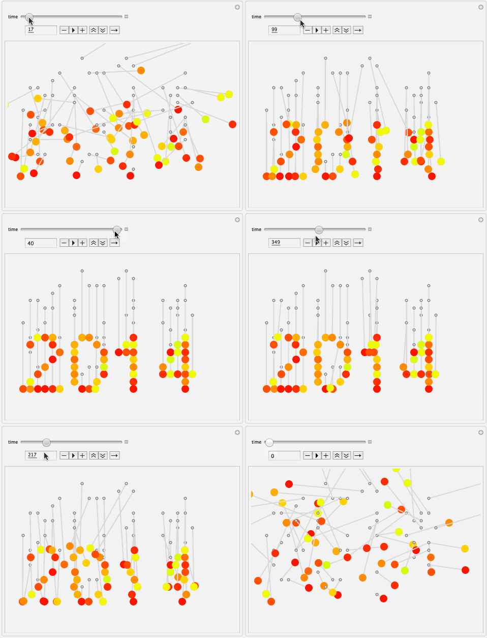
Finally ready to go greeting-manipulator
Manipulate[
Graphics[graphicsData[t], Background -> Lighter[Gray, 0.9],
PlotRange -> {{-1, 30}, {0, 22}}, ImageSize -> 550],
{{t, 0, "time"}, 0, 40, 1/48, AnimationRate -> 24, Appearance -> "Open"},
SaveDefinitions -> True, FrameMargins -> 0]
