Message Boards Message Boards

Solve a hypergeometric ODE NDSolve?

Posted 5 years ago

Eq1 = Dot[D[T[x], {x, #}] & /@ Range[0, 2], Factor@{1, D[-4 x (1 - x), x], -4 x (1 - x)}] == 0 ICs = MapThread[Equal, {(D[T[x], {x, #}] /. x -> 0) & /@ Range[0, 2], {1, 1/4, 9/32}}] Simplify[Eq1 /. MapThread[Rule, {D[T[x], {x, #}] & /@ Range[0, 2], D[2/Pi EllipticK[x], {x, #}] & /@ Range[0, 2]}]] Limit[D[2/Pi EllipticK[x], {x, #}], x -> 0] & /@ Range[0, 2]

This code validates that NDSolve on Eq1 & ICs should produce an interpolating function that returns values of EllipticK, but when I try:

NDSolve[Prepend[ICs, Eq1], T, {x, 0, 1}]

I get nonsense errors:

  • NDSolve::icordinit: The initial values for all the dependent variables are not explicitly specified. NDSolve will attempt to find consistent initial conditions for all the variables.
  • NDSolve::ndnco: The number of constraints (3) (initial conditions) is not equal to the total differential order of the system plus the number of discrete variables (2).

NDSolve not being able to solve a hypergeometric ODE seems like a "mission critical" error, so I'm feeling like an idiot while this call isn't working. Did I type something in wrong???

Thanks --Brad

POSTED BY: Brad Klee
3 Replies

Your differential equation is of the second order, but you give three initial data. Also, at the the starting point x==0 of the equation is singular:

NDSolve[{T[x] + 4 (-1 + 2 x) Derivative[1][T][x] + 
    4 (-1 + x) x (T^\[Prime]\[Prime])[x] == 0, T[0] == 1, 
  T'[0] == 1/4, T''[0] == 9/32}, T, {x,
   0, 1}]

DSolve gives a solution, which is probably equivalent with yours:

DSolve[Prepend[ICs, Eq1], T, x]
POSTED BY: Gianluca Gorni

Your differential equation is of the second order, but you give three initial data. Also, at the the starting point x==0 of the equation is singular

The error message asked for "initial values for all the dependent variables ", then complained that I gave three I.C.s, even though they are consistent. You are right that x=0 is a singular point, but why should this matter at all? Look at the graphs:

Plot[{ LegendreQ[-(1/2), -1 + 2 x], EllipticK[x]}, {x, -1, 1}, 
 PlotStyle -> {Directive[Lighter@Lighter@Blue, Thick], 
   Directive[Thick, Black, Dashing[.05]]}]

EllipticK

This particular solution is smooth at x=0, so iterative solution algorithms should work fine. In fact, the function EllipticK has a known series expansion, so if nothing else, the NDSolve could expand the series and evaluate. Also compare with:

ICs = MapThread[Equal,
   {(D[T[x], {x, #}] /. x -> 10^(-10)) & /@  Range[0,1], 
    (D[(2/Pi) EllipticK[x], {x, #}] /. x -> 10^(-10)) & /@ 
     Range[0, 1]}];
F = T /. NDSolve[Prepend[ICs, Eq1], 
    T, {x, 10^(-10), 1 - 10^(-15)}][[1]];
LogPlot[F[x] - 2/Pi EllipticK[x], {x, 0, .99}]

error

Using approximately x=0 as the initial condition, we can compute an accurate but imprecise solution. So it looks like we are getting closer, but we still don't know:

  • Is it possible to set the initial condition at x=0 and calculate a numerical solution to arbitrary precision? If yes, how? If no, why not?

Unfortunately, this is starting to look more like the "Mission Critical" failure I was worried about earlier.

POSTED BY: Brad Klee

How To: Calculate All Derivatives

Mat = Outer[Coefficient,
    D[Dot[{1, D[-4 x (1 - x), x], -4 x (1 - x)},
        {T[x], D[T[x], x], D[T[x], {x, 2}]}],
       {x, #}] & /@ Range[0, 10], D[T[x],
       {x, #}] & /@ Range[0, 11]] /. x -> 0;
Prepend[Mat, Prepend[Table[0, 11], 1]] // MatrixForm
LinearSolve[Prepend[Mat, Prepend[Table[0, 11], 1]], 
 Prepend[Table[0, 11], 1]]

out

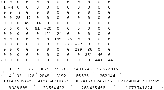
And notice, this acutally requires only one initial condition, not even two!

How To: DIY NDSolve

DerMat[n_] := Join[
   IdentityMatrix[n + 3][[1 ;; 2]],
   Outer[Coefficient,
    D[Dot[{1, D[-4 x (1 - x), x], -4 x (1 - x)},
        {T[x], D[T[x], x], D[T[x], {x, 2}]}],
       {x, #}] & /@ Range[0, n], D[T[x],
       {x, #}] & /@ Range[0, n + 2]]];

GetNext[mat_, cond_, dx_] := With[{Tx = Dot[
     LinearSolve[mat /. x -> cond[[3]], Join[cond[[1 ;; 2]],
       Table[0, Length[mat] - 2]]], 
     1/#! x^# & /@ Range[0, Length[mat] - 1]]
   }, {Tx, D[Tx, x], cond[[3]] + dx} /. x -> dx]

AbsoluteTiming[
 FApprox = Function[{MAT},
        Interpolation[
         NestList[GetNext[MAT, #, .0001] &, {1, 1/4, 0}, 
           9999][[All, {3, 1}]]]][DerMat[#]] & /@ {2, 3, 4, 5, 6} // 
    Quiet;]

Show[LogPlot[
    Abs[FApprox[[#]][x] - 2/Pi EllipticK[x]], {x, .001, .9999}, 
    PlotRange -> All, 
    PlotStyle -> {Red, Orange, Yellow, Green, Blue}[[#]]] & /@ 
  Range[5],
 LogPlot[10^(-#), {x, 0, 1}, PlotStyle -> Black] & /@ {7, 11},
 PlotRange -> All]

err2

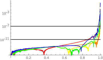
Compare with earlier error plot. This quick hack is already doing better than NDSolve, and accepts initial condition at x=0. Any thoughts?

POSTED BY: Brad Klee
Reply to this discussion
Community posts can be styled and formatted using the Markdown syntax.
Reply Preview
Attachments
Remove
or Discard

Group Abstract Group Abstract