Introduction
Recently, I was learning about infinite space filling curves and their applications in real life. I became fascinated with Hilbert Curves, one of many plane-filling functions. I wanted to see how these shapes could be used in image to video conversion. To begin with, I explored how pseudo Hilbert Curves could be used to convert a square image to audio so that each pixel color was associated with a specific sound.
Theoretically, a person would be able to learn this association and would be able to reconstruct a mental image by listening to audio. This could help with people who are visually impaired, letting blind people "hear" pictures. The reverse is also true. People who are deaf will be able to "see" sound.
I thought I could implement this using Mathematica, which I learned last summer at the Wolfram High School Camp.
Why Hilbert Curves
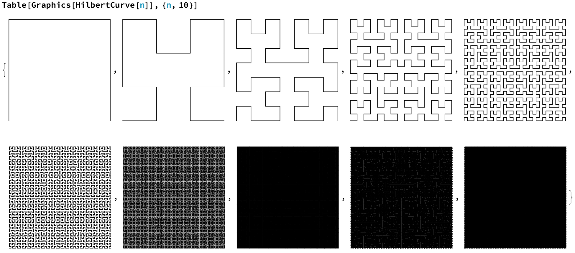 As you can see above, as you increase the order, the limit of these curves start to fill an infinite amount of space. A true Hilbert Curve is actually $\lim_{n\to\infty} PseudoHilbertCurve_n$. Each one of these curves can be used on an image of dimensions 2 by 2, 4 by 4, 8 by 8, etc. The curve needed is accordingly:
HilbertCurve[Log[2, ImageDimensions[image]]]
Each line in the curve will go over one pixel in the image, starting at the bottom left and ending at the bottom right.
But why would you need to use this specific pattern, as supposed to something more simple? Here: https://youtu.be/3s7h2MHQtxc?t=355. In short, if you were to increase the resolution of your image, you would now have to retrain your brain to re-associate the pixel value and the associated frequency at that point on the image. But this is not the case on a Hilbert Curve. As you increase the resolution of your image, and thus the order pseudo-Hilbert Curve, a point will just move closer and closer to its limit in the same space, which solves our problem.
Converting Color to Sound
This was the main hurdle when writing the program. I needed to convert each pixel value to a unique sound frequency. My initial thought was to just create an association between each wavelength in the visible electromagnetic spectrum and a frequency, but I was quick to learn that doesn't work in the digital world. RGB colors could be a combination of different wavelengths. And I couldn't just add these wavelengths separately because there could be overlap. There was also brightness and darkness which isn't part of the light spectrum. So instead of the RGB format, I decided to use the HSB format (hue, saturation, and brightness). This is also more compatible for human learning, as the human eye uses these three characteristics to determine color, as supposed to the RGB values on a computer image.
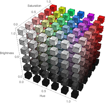
As you can see from the image, Hue could be used to determine the color. Now, instead of RGB with three values to one color, Hue gave me one number to a specific color.

But I still needed to show saturation and brightness in my sound waves. Color in a computer is expressed in three dimensions while sound has two: amplitude and frequency. I would be leaving one color property out. I could think of multiple ways to express all three as sound waves, but none of them made sure that similar colors sounded the same. For example, if I had a hue playing a certain frequency, I could define a range around this point that could express either saturation or brightness using a plus/minus system.
To solve this, I decided to use AudioChannel functions. This way, one channel could express the hue through a specific frequency, while the other channel could express the saturation and brightness combined through volume and frequency respectively. This way, colors that were similar would sound similar too.
Creating the Function
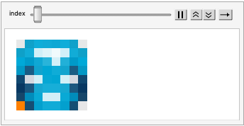
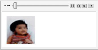
Obviously, I needed to get real images. I used image1, where the pixels were easily noticeable, and my baby picture for the school yearbook as image2, as a test image. The first one, being resized to a 8 by 8 image, would utilize an order 3 pseudo-Hilbert Curve ( $\log _{2}8=3$), and the second one, being resized to a 32 by 32 image, would utilize an order 5 pseudo-Hilbert Curve ( $\log _{2}32=5$).

To get the HSB values, I used Wolfram's in-built Hilbert Curve and Pixel Value functions. I used Pixel Value to read the image's pixel values as bytes, which was converted to RGB and then to HSB. To get the points on the Hilbert Curve that was associated with their respective position on the image, I added {1,1} to each point so that it matched the pixel space (the origin on a Cartesian Plane is designated as (1,1) on an image).
getHSB[image_] :=
 ColorConvert[
  RGBColor /@
   Divide[PixelValue[
     image, ({1, 1} + #) & /@
      HilbertCurve[Log[2, ImageDimensions[image][[1]]]][[1]], "Byte"],
     255.], "HSB"]
In the Wolfram Language, HSB values range from 0 to 1 instead of the normal 0 to 360 which I guess gives the user more control of the specific color they want to implement. I had to scale these values to the frequency range I wanted for the hue and brightness. Through trial and error, I decided that 100-3900 Hz was a good range so that people of all ages could hear the lowest and highest frequencies. For the amplitude dictated by the saturation, I could just use the direct value as SoundVolume. I made it so that the sound for each pixel had a duration of 0.1 seconds for demonstrative purposes. In the real world, I would think that this should be a lot smaller so that images don't take too long to hear.
getHSB[image_] :=
 ColorConvert[
  RGBColor /@
   Divide[PixelValue[
     image, ({1, 1} + #) & /@
      HilbertCurve[Log[2, ImageDimensions[image][[1]]]][[1]], "Byte"],
     255.], "HSB"]
hueToFrequencyMatch[HSB_] := Rescale[HSB[[1]], {0, 1}, {100, 3900}]
saturationToAmplitudeMatch[HSB_] := HSB[[2]]
brightnessToFrequencyMatch[HSB_] :=
 Rescale[HSB[[3]], {0, 1}, {100, 3900}]
soundFrequency[frequency_] :=
 Sound[Play[Sin[frequency*2 Pi t], {t, 0, 0.1}]]
soundFrequencyVolume[frequency_, ampSaturation_] :=
 Sound[soundFrequency[frequency], SoundVolume -> ampSaturation]
After this, I just had to apply these functions over the HSB values of each pixel in the order dictated by the appropriate pseudo-Hilbert Curve, and then merge the hue sound and saturation+brightness sound as separate audio channels.
convertHToSound[image_] :=
 soundFrequency /@ hueToFrequencyMatch /@ getHSB[image] // AudioJoin
convertBSToSound[picture_] :=
 (soundList = {}; n = 1;
  While[n <= Length@getHSB[picture],
   AppendTo[soundList,
    soundFrequencyVolume[
     getHSB[picture][[n]] // brightnessToFrequencyMatch,
     getHSB[picture][[n]] // saturationToAmplitudeMatch]];
   n++])
convertHSBToSound[audio1_, audio2_] :=
 AudioChannelCombine[{audio1, audio2}]
Because hue is the most important color characteristic, I wanted to emphasize this AudioChannel more. Thus,
editChannel2[audio_, factor_] := AudioPan[audio, -factor]
To put everything together, I made a separate function to organize the results.
seperateTable[picture_] :=
 (convertBSToSound[picture];
  Module[{a = convertHToSound[picture], b = soundList // AudioJoin},
   c = editChannel2[convertHSBToSound[a, b], 0.05];
   table =
    Grid[{{Image[picture, ImageSize -> 100], a, b, c}, {Blank[],
       AudioPlot@a, AudioPlot@b, AudioPlot@c}}];
   ReplacePart[table,
    1 -> Prepend[
      First[table], {"Image", "Hue", "Saturation+Brightness",
       "HSB"}]]])
These were my results. I will attach the hsb1 and hsb2 sound files to this post, along with my notebook.
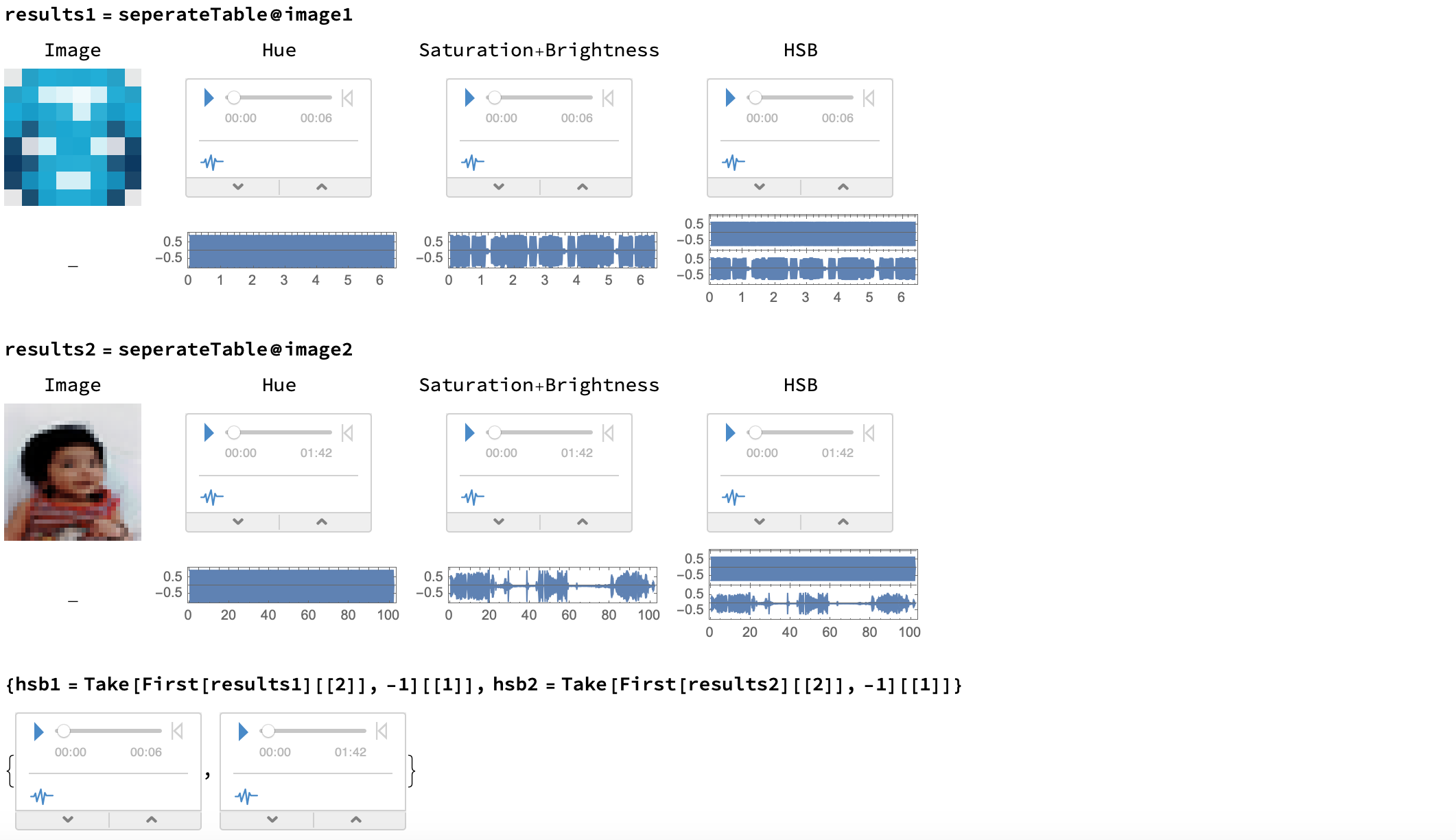 Because they use two channels, you should use earbuds or headphones so that you can clearly differentiate the sounds coming through your left and right ears.
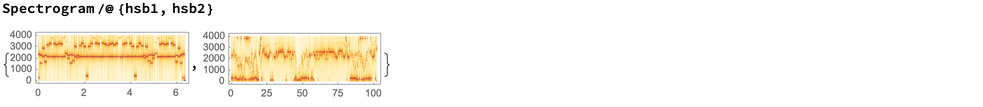
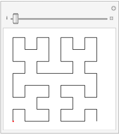
Visualizing the Process
animate[image_, audio_] :=
    Module[{list = ({1, 1} + #) & /@
    HilbertCurve[Log[2, ImageDimensions[image][[1]]]][[1]]},
  (AudioPlay@audio;
   Animate[
    ReplacePixelValue[Image[image, ImageSize -> 100],
     list[[1 ;; index]] -> Orange],
    {index, 1, list // Length, 1},
    DefaultDuration ->
     QuantityMagnitude[
      UnitConvert[Quantity[audio // Duration, "Seconds"]]],
    AnimationRepetitions -> 1])]
I used this to create the following two animations. If you ran these programs, the HSB sound would play alongside the animation, showing exactly which pixel correlates to each sound. Unfortunately, I couldn't play the audio here on the post, but it is in the attached notebook if you would like to see. Here is what it looks like:
Future Work
In the future, I hope to create a machine learning algorithm that can learn this association between audio and image in reverse (recreate the image from audio). If anyone has any ideas or pointers for me, please share in the comments below - I would really appreciate it!
Updated Information:
Presented work at the New Hampshire Science & Engineering Expo and won the Office of Naval Research award.
Youtube Link: Video Presentation
 Attachments:


