See,
The Wolfram Language includes Parallel Computing Tools, and parallel computing is the first step in high-performance computing. The combination of parallel computing tools and object-oriented programming (following OOP here) introduces a new perspective on Wolfram Language programming. OOP is well-suited for parallel computing because instances are essentially independent computational units and the same code can be applied in both parallel and mono-kernel environments.
So far, the author has introduced an OOP system for the Wolfram Language, and continues with Part 1 and 2 with examples of OOP-based parallel computing.
Part 3 is concerned to the calculations using large-sized instances such as 10^6 deployed on the multi local cores. This example is intended to parallel nearest points calculation for 10^6 points randomly dispersed in a 3d area. The example is based on the case of 4 local CPU cores.
Parallel code efficiency is depend on the CPU performance and multi-core performance, you should implement this sample code on your computer and then can evaluate this OOP methods. This sample has shown that the OOP parallel computing efficiency is scaling to the number of CPU cores, then the Wolfram OOP code for the newest CPUs will show an excellent performance, if the ParallelEvaluate[] function can handle greater number of cores which is limited in the present version of Wolfram language.
step.1 setup local kernels
LaunchKernels[];
kernelList = ParallelEvaluate[$KernelID];
nk = Length[kernelList];
kernelNameList = Table[Unique[k], {nk}];
step.2 definition of parallel calculation class, You can find nested class in the following code which defines the parallel calculation class. Each instance constructed form this class simply holding the position of itself given randomly at the time of construction.
kernel[nam_] := Module[{myKernelName = nam, prNameTable},

       (* define parallel calculation class *)

       para[pnam_] := Module[{pos = RandomReal[1, 3]},
         getpos[pnam] := pos];

       (* kernel method to make parallel calculation object list *)

       setprtable[n_] := prNameTable = Table[Unique[c], {n}];

       (* kernel method to construct parallel calculation instances using \
    object list *)
construct[] := Map[para[#] &, prNameTable];

       (* nearest calculation method *)
       near[x_, n_] := Nearest[Map[getpos[#] &, prNameTable], x, n]
       ];
step.3 definition of the number of parallel calculation instances on each core. In this case, total number of instances is 10^6= 4*250000.
nInstance = 250000;
step.4 definition of local kernel property
kernelObject =
 Table[Association["name" -> kernelNameList[[i]],
   "kernel" -> kernelList[[i]]], {i, nk}]
step.5 constructing local kernel instances with predefied association list,
AbsoluteTiming[
 Map[ParallelEvaluate[kernel[#name], #kernel] &, kernelObject]
 ]
step 6. accessing to the method of local kernel instances, preparing the name list of parallel computing instances in parallel
AbsoluteTiming[
 ParallelEvaluate[setprtable[nInstance]];]
step 7. accessing to the method of local kernel instances, to construct and deploy the parallel computing instances
That is, on each core, instances will be constructed in parallel.
AbsoluteTiming[
 ParallelEvaluate[construct[]];]
step 8. execution of parallel computing
AbsoluteTiming[
 ans = ParallelEvaluate[near[{0.5, 0.5, 0.5}, 10]]]
Results of computation
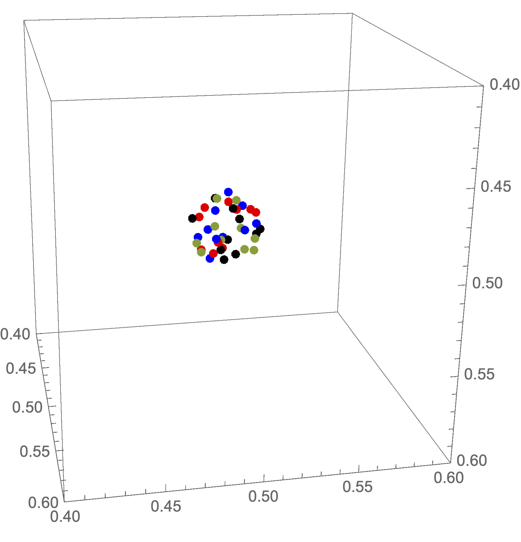
Following 3D graphics shows each nearest 10 points calculated on each core near zero-point {0.5,0.5,0.5}.
ListPointPlot3D[{ans[[1]], ans[[2]], ans[[3]], ans[[4]]},
 PlotStyle -> {Red, Blue, Greem, Black},
 PlotRange -> {{0.4, 0.6}, {0.4, 0.6}, {0.4, 0.6}},
 BoxRatios -> Automatic]
