MODERATOR NOTE: Wolfram notebook is attached at the end of the post.

In memory of John Horton Conway, 1937-2020

John Horton Conway, described by Michael Atiyah as "the world's most magical mathematician", was one of the most brilliant and playful mathematicians of our time. In his career, he studied a diverse array of subjects, from abstract algebra, with Monstrous Moonshine, to geometry, with Conway Polyhedral Notation, and most famously, mathematical computing and game theory, with his eponymous Game of Life. Perhaps one of his most curious (and certainly less well-known) contributions is what he called the Audioactive, (or Cuckoo's Egg) sequence.

The Audioactive Sequence

To explain the sequence, it is best to propose a riddle (which is how it is often proposed).

What comes next in the sequence: 1, 11, 21, 1211, 111221, 312211 ... ?

If you have not seen this before, take a moment to think about this before reading further.

The answer, of course, is 13112221 - the sequence is made by reading aloud the previous term, like you would a phone number - hence, audioactive. For example, 111221 would be read as 'three ones, two twos and one one' - hence, 312211.

You may be wondering about where the Mathematica comes in. Have patience.

Firstly, the sequence in code:

In[1]: audioactive[list_] := Flatten[{Length[#], #[[1]]} & /@ Split[list]]

To test it out (in colour, which makes it a lot easier to see):

In[2]: styled[string_, colour_] := 
 Style[string, FontFamily -> "Courier New", FontSize -> 50, 
  FontColor -> colour]; digits = <|1 -> styled["1", Red], 
  2 -> styled["2", Green], 3 -> styled["3", Blue]|>;

In[3]: SetDirectory[NotebookDirectory[]]; 
    Export["sequence1.gif", 
 Row[digits[[#]] & /@ #] & /@ NestList[audioactive, {1}, 10], 
 "AnimationRepetitions" -> \[Infinity], 
 "DisplayDurations" -> Table[.5, 11]];
 (*I did try GraphicsRow, but this didn't seem to work - 
    if anyone can explain, please comment*)

which returns

One interesting observation to be made is that there appear to be no 4s here - the only digits are 1s, 2s and 3s. `Even if we did start with a 4, observe what happens to it:

In[4]: Export["sequence2.gif", 
 Row[Join[digits[[#]] & /@ #[[;; -2]], {Style["4", 
       FontFamily -> "Courier New", FontSize -> 50, 
       FontColor -> Purple, FontWeight -> Bold]}]] & /@ 
  NestList[audioactive, {4}, 10], 
 "AnimationRepetitions" -> \[Infinity], 
 "DisplayDurations" -> Table[.5, 11]];

Any number larger than four will stay in the same relative position - for the most part, they are entirely irrelevant. In fact, unless the first sequence contains a 4 or higher, or a string of 4 identical numbers, then the numbers 4 and higher will never appear (which, in true mathematical style, is left as an exercise to the reader) - that is, a 4 can only occur later than the second iteration (or "day" as Conway calls it) if it has occurred in the first two days. This is known as the Two Day Theorem (this wonderful biochemistry article, which was thankfully retrieved, talks about this, and the rest of the article in much greater depth, as well as showing the connection between this and RNA sequences - fascinating). From here on in, we will only consider sequences comprising of 1s, 2s and 3s.

Conway's Constant

One question which might be asked is how the length of the sequence behaves, especially from an asymptotic perspective. Let us begin with a sequence beginning with "1":

In[5]: lengths1 = Length /@ NestList[audioactive, {1}, 25];

In[6]: ListLinePlot[lengths1]

which returns

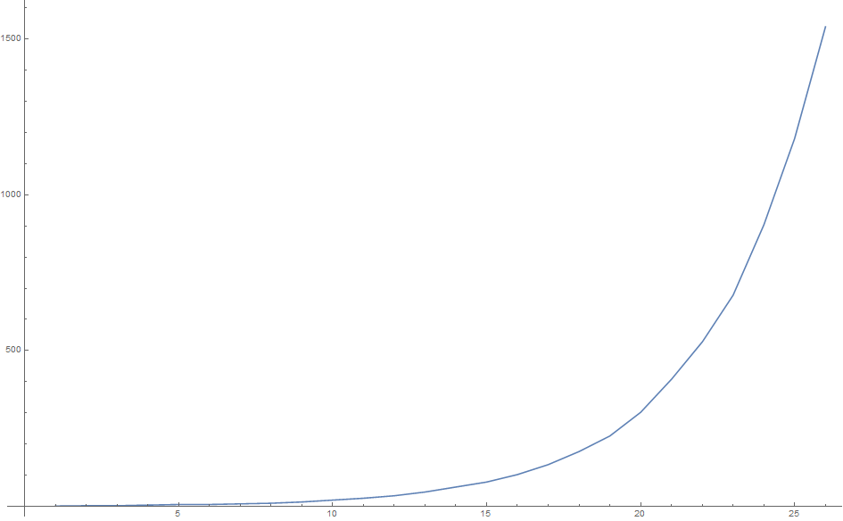
It is very clear that this is an exponential curve - so, it's natural to take a look at the ratios of the sequence lengths.

Let's look at another starting sequence, and compare this on a logarithmic plot:

In[7]: lengths2 = Length /@ NestList[audioactive, {1, 3, 2}, 25];

In[8]: ListLogPlot[{lengths1, lengths2}, Joined -> True]

giving

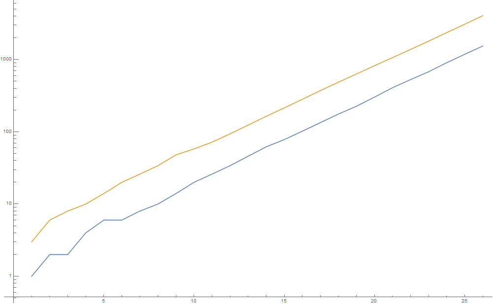
It looks like both curves eventually have the same gradient - that is, the ratio of the consecutive lengths reaches the same value eventually. So, it would be reasonable to conjecture that:

There exists some $\lambda$ such that, for almost all sequences, there exists some constant $C$ such that, after n days, the length of the sequence is asymptotically equal to $C \cdot \lambda^n$

Here, "almost all" turns out to be all sequences of digits, with the exceptions of the empty sequence and the sequence 22 (which just repeats forever). The value of $\lambda$ (which is known as Conway’s constant) can be estimated quite easily:

In[9]: N[lengths1[[-1]]/lengths1[[-2]]]

Out[9]: 1.30288

But what is the exact value of Conway's constant?

Example - Fibonacci words

Define a sequence (which is significantly simpler to analyse compared to Conway's one), to start with A (or any other sequence of As and Bs, for that matter), and substitute an A for a B, and a B for an AB.

In[10]: fibonacciWord[list_] := Flatten[list /. {"A" -> "B", "B" -> {"A", "B"}}]

In[11]: letters = <|"A" -> styled["A", Red], "B" -> styled["B", Green]|>;

In[12]: Export["sequence3.gif", 
 Row[letters[[#]] & /@ #] & /@ NestList[fibonacciWord, {"A"}, 8], 
 "AnimationRepetitions" -> \[Infinity], 
 "DisplayDurations" -> Table[.5, 9]];

giving The astute amongst you may notice that the lengths of the sequence are Fibonacci numbers. Observe that, if we have a vector consisting of the number of As and the number of Bs in the sequence, say, $\begin{pmatrix} \#A \\ \#B \end{pmatrix}$, then by the definition of our sequence, after one iteration, we will end up with $\begin{pmatrix} 0 & 1 \\ 1 & 1\end{pmatrix} \cdot \begin{pmatrix} \#A \\ \#B \end{pmatrix}$. If we assume the ratios between the number of As and number of Bs will eventually converge to some vector, $\begin{pmatrix} p_A \\ p_B \end{pmatrix}$, this will be an eigenvector of the matrix - since it will get mapped into the same proportions. If the eventual ratio of lengths is some $\phi > 1$, then this will be mapped to $\begin{pmatrix} \phi \cdot p_A \\ \phi \cdot p_B \end{pmatrix}$ - so it is the eigenvalue of the vector (and therefore, a root of the characteristic polynomial of the matrix - sorry if this is getting a bit linear algebra-y).

In[13]: matrix = {{0, 1}, {1, 1}};

In[14]: Eigenvalues[matrix]

Out[14]: {1/2 (1 + Sqrt[5]), 1/2 (1 - Sqrt[5])}

The only positive value here is $\frac{1+\sqrt{5}}{2}$, better known as the Golden Ratio (which is also the ratio between consecutive terms of a general Fibonacci sequence). This is exactly what we are going to try here.

There is a problem, though: this isn't a simple substitution system like the Fibonacci words. So how can we use this trick to find the value of Conway's constant?

Conway's Cosmological Theorem

In a stroke of genius, Conway had an idea - try to find long sequences, called elements, which will eventually decompose into other elements. The crux was to show that every sequence will eventually decay into one of these elements (which, in characteristic good humour, were named after chemical elements, from Hydrogen to Plutonium). This lead to the Cosmological Theorem:

Theorem: After 24 days, every sequence will decay into a concatenation of common and transuranic (i.e, Plutonium and Neptunium) elements.

(A proof of this can be found in this paper by Ekhad and Zeilberger - interestingly, it was proven using a computer for the most part; the original proof by Conway has unfortunately been lost). This will not be proven here, nor will it be set as an exercise to the reader - it took hundreds of lines of code to prove (I guess it was Maple in 1998, though); it may be another Mathematica project for a later date...

Calculating Conway's Constant

The biochemistry article turns out to have pre-computed the sequences and "decays" of the elements, in Appendix 4; the raw text from this is in attachment. In keeping with the "ignore all values greater than 3" policy, I have removed both tranuranic elements - since these specifically deal with the such digits.

Firstly, basic text manipulation:

In[15]: rawElements = Association[#[[2]] -> {#[[3]], 
      StringSplit[#[[4]], DigitCharacter] /. "" -> Nothing} & /@ 
   Partition[
    StringSplit[
     Import["elements.txt"]], 4]];

All this does is converts the text file format from number, element, sequence, decays, into the more useful element -> {sequence, decays}. Next, this kind of dataset is begging to be drawn as a graph - so this is what we shall do.

In[16]: labels = (# -> Tooltip[Framed[#], Entity["Element", #]]) & /@ 
 Keys[rawElements];

In[17]: graph = Graph[Flatten[
  Table[#[[1]] -> #[[2, k]], {k, Length[#[[2]]]}] & /@ 
   List @@@ Normal@(#[[2]] & /@ rawElements)], VertexLabels -> labels, 
 VertexLabelStyle -> 15]

returning this:

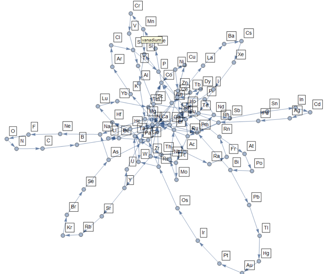
with the handy mouse-over property. Observe that, for the most part, elements decay by 1 each time - for example, Manganese decays to Chromium, which in turn decays to Vanadium (my favourite element). There are some exceptions to this - for example, Hydrogen, which just decays into itself.

Another useful representation of graphs is the adjacency matrix, $(m_{u,v})_{u, v \in V}$ - where element $m_{u,v}$ counts the number of directed paths from u to v. (This is analagous to the matrix discussed in the Fibonacci Words section), which is best described as an Array Plot:

In[18]: AdjacencyMatrix[graph] // ArrayPlot

giving: 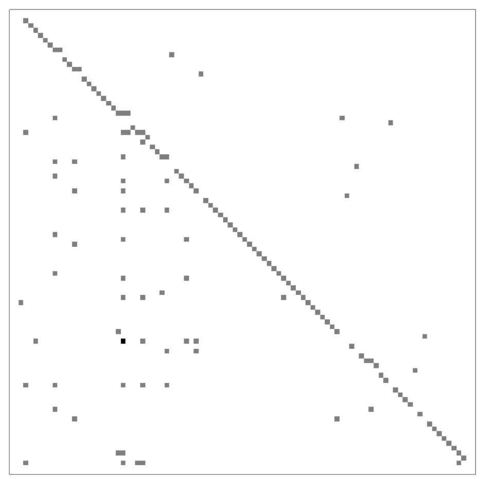which gives a clearer indication as to how the elements tend to decay. Let us plot the eigenvalues, highlighting those which are real and greater than one in red:

In[19]: eigs = Eigenvalues[AdjacencyMatrix[graph]];

In[20]: ComplexListPlot[{eigs, Select[eigs, Positive[# - 1] &]}, 
 Axes -> False, PlotMarkers -> {"\[Times]", 15}, 
 PlotStyle -> {Black, Red}]

returning

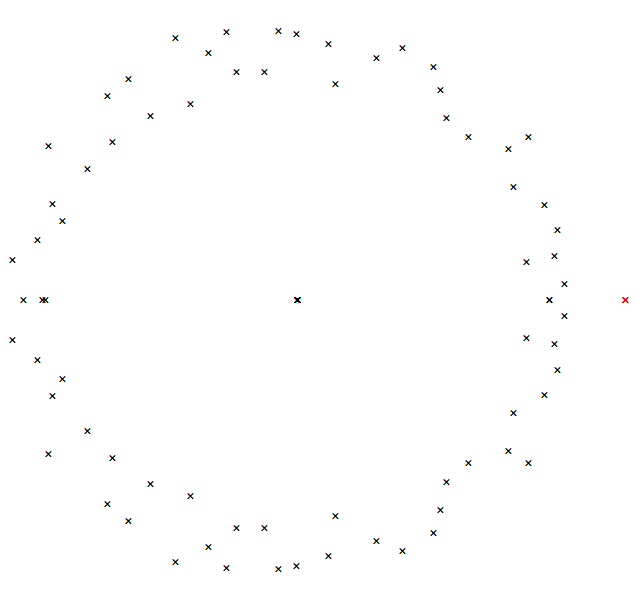
There is only one red cross.

This is Conway's constant.

In[21]: \[Lambda] = Select[eigs, Positive[# - 1] &][[1]];

To 100 decimal places:

In[22]: N[\[Lambda], 100]

Out[22]: 1.30357726903429639125709911215255189073070250465940487575486139062855\
0887852461557126815766864425226

Since this is the root of the characteristic polynomial, it is not transcendental; its minimal polynomial is:

In[23]: MinimalPolynomial[\[Lambda], t]

Out[23]: -6 + 3 t - 6 t^2 + 12 t^3 - 4 t^4 + 7 t^5 - 7 t^6 + t^7 + 5 t^9 - 
 2 t^10 - 4 t^11 - 12 t^12 + 2 t^13 + 7 t^14 + 12 t^15 - 7 t^16 - 
 10 t^17 - 4 t^18 + 3 t^19 + 9 t^20 - 7 t^21 - 8 t^23 + 14 t^24 - 
 3 t^25 + 9 t^26 + 2 t^27 - 3 t^28 - 10 t^29 - 2 t^30 - 
 6 t^31 + t^32 + 10 t^33 - 3 t^34 + t^35 + 7 t^36 - 7 t^37 + 7 t^38 - 
 12 t^39 - 5 t^40 + 8 t^41 + 6 t^42 + 10 t^43 - 8 t^44 - 8 t^45 - 
 7 t^46 - 3 t^47 + 9 t^48 + t^49 + 6 t^50 + 6 t^51 - 2 t^52 - 
 3 t^53 - 10 t^54 - 2 t^55 + 3 t^56 + 5 t^57 + 
 2 t^58 - t^59 - t^60 - t^61 - t^62 - t^63 + t^64 + 2 t^65 + 
 2 t^66 - t^67 - 2 t^68 - t^69 + t^71

a 71st degree polynomial. Since the polynomial has leading coefficient 1, and $\lambda$ is not integer, by the Rational Root Theorem, it must be irrational.

Finally, what are the relative proportions of 1s, 2s and 3s? All we need for this, as we saw earlier, is the eigenvector associated with this.

In[24]: vector = First@NullSpace[
  N[AdjacencyMatrix[graph] - \[Lambda]*IdentityMatrix[92]]];

Next, to count the number of characters in each element:

In[25]: count[char_] := 
 Count[Characters[First[#]], char] & /@ Values[rawElements]

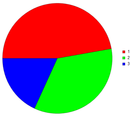
In[26]: proportions = 
 Normalize[{count["1"].vector, count["2"].vector, count["3"].vector}, 
   Total]*100

Out[26]: {47.1995, 34.6579, 18.1426}

So, we should expect to see significantly more 1s and 2s than 3s - in fact, nearly half of all the digits can be expected to be a 1. In a pie chart, using the same colour scheme as earlier:

In[27]: PieChart[proportions, ChartLegends -> {"1", "2", "3"}, 
 ChartStyle -> {Red, Green, Blue}, LabelingSize -> 100]

which gives:

If the sequence tended to infinity, and all we saw was a blur, the colour we would see would be:

In[28]: RGBColor[proportions/100]

which returns a rather unpleasant shade of brown. Oh well.

In memoriam, John Horton Conway, 1937 - 2020

Attachments:

audioactive.nb

elements.txt