Message Boards Message Boards

0
|
10460 Views
|
12 Replies
|
3 Total Likes
View groups...
Share
Share this post:

Siemens sine-wave stars

Posted 4 years ago

Hi Wolframians, I am new to the Wolfram language, and I only used a trial version of the Mathematica to see if there is a way to replace my Siemens sine-wave star measurement for my test chart, using MatLab. I am under impression that Mathematica is much more powerful, but as with anything new, it is hard for me to find a function or algorithm of how I can measure resolution of a Siemens sine-wave star, which I use in my ViDi Labs test charts (https://vidilabs.com/testcharts.html) and developed a little program using MatLab to find the circles in an image, and then measure resolution (or MTF = Modulation Transfer Function), based on the 10% Depth of Modulation, as described by the IEC 62676-5 standards. If anybody can help me in either giving me a list of functions to look at, or perhaps somebody would know exactly how to calculate the above mentioned resolution, I would gladly purchase a full licence of Mathematica and investigate this further. Happy to consider even paying somebody for their time if they can do what I have described in my video in the able mentioned URL link. I am also adding an attachment, a simple explanation on how this resolution is measured. Thank you so much.

Attachment

Attachments:
12 Replies

I am under impression that Mathematica is much more powerful ...

Your impression is absolutely correct! Here comes an attempt showing some intermediate result which hopefully points to the right direction:

First I create an image of a Siemens star; its center is "somewhere":

siemensFunc[x_, y_] := (Sin[144 ArcTan[x, y]] + 1)/2.
ll = 5.01;
siemensStarData = Table[siemensFunc[x, y], {y, -ll, ll + 1, .02}, {x, -ll + 1, ll + 1, .02}];
siemensStar = Image[siemensStarData]

Now I am taking this image as it is. To get the star center I first try to find "lines" in the image:

lines = ImageLines[siemensStar];
HighlightImage[siemensStar, lines]

enter image description here

and calculate the mean value of some of the crossings:

linePairs = Partition[lines, 2, 1];
center = Mean[(RegionIntersection /@ linePairs)[[All, 1, 1]]]

Knowing the center circles can be drawn:

circles = Table[Circle[center, r], {r, 15, 300, 30}];
HighlightImage[siemensStar, circles]

enter image description here

POSTED BY: Henrik Schachner

I think it is not really clear what you want to do. What exactly is your problem?

POSTED BY: Hans Dolhaine

Ok Hans, this is what i would summarise it as: 1. A test chart has 5 Siemens stars, one larger one in the centre and four smaller in each corner. An image is taken by a camera and exported as JPG or BMP. How would you find the five circles and their centres? 2. Once the circles are found and their respective centres, one needs to measure the Depth of Modulation, as per the image I attached previously. Basically find how close to the centre the B/W rays are distinguishable with 10% contrast. 3. Based on the measurement under 2 (In pixels) calculate the MTF expressed in Line Pairs per Picture height. This is admittedly very easy if 1 and 2 are automated. I have attached a real camera export, which means they could always be slight variations in star positions, their geometry could be distorted (not always perfect circles) and have different resolution (which is to be measured).

I understand you have an image (as bitmap). This is an ( n, m ) array of bytes, and as first step you want to find those regions which show siemens stars?

This seems to be a question for experts in image-analysis or image-processing.

POSTED BY: Hans Dolhaine

Vlado, this seems to be an interesting topic, but without any typical test image it is hard to say anything.

A test chart has 5 Siemens stars, one larger one in the centre and four smaller in each corner. [...] I have attached a real camera export ...

So, where is it?

POSTED BY: Henrik Schachner

Thank you Hans, thank You Henrik, The last response from Henrik seems to be what I am after, and it is very promising. I am not sure why you didn't see the original image I had attached in my last response, as I used the "Add file to the post". But I am now attaching the original real export of a CCTV camera (typically they are HD or 4k resolution) and the measurements that I have made using Matlab. As you can see I am also measuring other parameters of the reproduced test chart, like the colour, Gamma and noise. I am not very happy with the Siemens star measurements, as they are not consistent with what I measure manually using PhotoShop for example. This is the reason I intend to try Mathematica, which I have no experience with, but willing it to try. I am assuming, finding the colour coordinates of the colour patches would be easy, and so would the random pixel noise of a grey patch representing 50% grey. Thank you very much for this hint Henrik, I will try and reproduce it myself on the real test chart and calculate the Depth of Modulation.

Attachment

Attachment

Attachment

As usual Henrik is far ahead.

Here is a first attempt to find a (simple) circular structure in an image. First make the image. Define its limits and what else is needed

x1 = 3;
x2 = 9.8;
y1 = -.2;
y2 = 10;
rr = 1.35;
xc = 5;
yc = 4;
col = {.2, .7, .1};

Then show it

pl1 = Graphics[Disk[{xc, yc}, rr],
  Background -> RGBColor[col],
  PlotRange -> {{x1, x2}, {y1, y2}}]

Extract the informtion embedded in the image

dat = ImageData[pl1];
dim = Dimensions[dat]

Find the y-position of the centre of the disk, assuming the disk is black

d1 = Count[#, {0., 0., 0.}] & /@ dat
ymm = Flatten[Position[d1, Max[d1]]]
ym = Floor[Mean[ymm]]
yccalc = y2 + (ym - 1)/(dim[[1]] - 1) (y1 - y2)

and the same for x and the radius

posxblack = Flatten[Position[dat[[ym]], {0., 0., 0.}]]
dia1 = Last[posxblack] - First[posxblack]
xm = Floor[Mean[posxblack]]
xccalc = x1 + (xm - 1)/(dim[[2]] - 1) (x2 - x1)
radcalc = dia1 /dim[[2]] (x2 - x1)/2

Show what we have found in comparison to the original data

pl2 = Graphics[
  {Blue, Disk[{xccalc, yccalc}, radcalc]},
  PlotRange -> {{x1, x2}, {y1, y2}}]
Show[pl1, pl2]

This code should be checked with different settings for the parameters of the picture, which I haven't done yet.

And I am not sure how to extend this to find a Siemens star like that given in your very first pic above.

POSTED BY: Hans Dolhaine

Vlado, here comes a slight extension:

First - as a side note - here is an improved siemensFunc:

siemensFunc[phases_Integer, px_, x_, y_] := Module[{r, \[Phi], rlim},
  If[(x == 0) && (y == 0), Return[0]];
  r = Norm[{x, y}];
  \[Phi] = ArcTan[x, y];
  rlim = px phases/Pi;
  If[r > rlim, (Sin[phases \[Phi]] + 1)/2., (Sign[Sin[-2 \[Phi]]] + 1)/2.]
  ]

ll = 5.01;
px = 0.02; (* pixel size *)
siemensStarData = Table[siemensFunc[120, px, x, y], {y, -ll, ll + 1, px}, {x, -ll + 1, ll + 1, px}];
Image[siemensStarData]
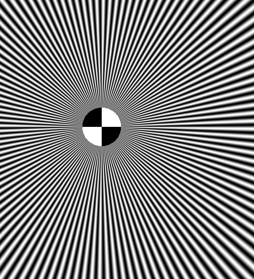
enter image description here

But my remark here is basically about processing the test image you sent, and the main thing is a hopefully more robust function for finding the star centers:

findSiemensStarCenter[img_Image] := 
 Module[{star, lines, linePairs, intersects},
  star = SelectComponents[Binarize[img], #EnclosingComponentCount == 1 &];
  lines = ImageLines[Binarize@star, MaxFeatures -> 15];
  linePairs = Partition[lines, 2, 1];
  intersects = (RegionIntersection /@ linePairs) /. EmptyRegion -> Nothing;
  TrimmedMean[intersects[[All, 1, 1]], .2]
  ]

SetDirectory[NotebookDirectory[]];
(* assuming that your MMA notebook and the test image are in the same directory *)
testImg = Import["20191119_164554.bmp"];

(* extracting the 5 Siemens stars: *)
{dimx, dimy} = ImageDimensions[testImg];
parts = ImagePartition[testImg, {dimx/5, dimy/3}];
{topleft, topright, bottomleft, bottomright} = Extract[parts, {{1, 1}, {1, 5}, {3, 1}, {3, 5}}];
middle = ImageCrop[testImg, {700, 700}];

(* calculating its centers: *)
centers = findSiemensStarCenter /@ {topleft, topright, middle, bottomleft, bottomright}

You can concentrate all this using an Association:

siemensStars = 
  Association[
   "TopLeft" -> Association["Image" -> topleft, "Center" -> centers[[1]]], 
   "TopRight" -> Association["Image" -> topright, "Center" -> centers[[2]]],
   "Middle" -> Association["Image" -> middle, "Center" -> centers[[3]]], 
   "BottomLeft" -> Association["Image" -> bottomleft, "Center" -> centers[[4]]], 
   "BottomRight" -> Association["Image" -> bottomright, "Center" -> centers[[5]]]];

and than you can do things like siemensStars["BottomRight", "Center"] or siemensStars // Dataset. And you can convince yourself about the correctness of the above calculation like so:

cccircles[center_] := Table[Circle[center, r], {r, 15, 500, 30}]
Grid[KeyValueMap[{#1, HighlightImage[#2["Image"], cccircles[#2["Center"]]]} &, siemensStars], Frame -> All]

enter image description here

Maybe this serves as an inspiration.

POSTED BY: Henrik Schachner

Wow Henrik, I am impressed, although I am yet to start using your inspirational suggestions :-). Do you mind writing me a direct e-mail to vlado@vidilabs.com so I can give you some other material for you to look at which would be difficult to include here as attachment. But only if you have time and willing to continue with your suggestions :-)

Thank you kindly Henrik.

Hi Vlado, sorry for the delay! Here is a sketch of my approach for finally calculating the MTF (according to the formula you gave). I am assuming we have defined the above siemensStars association, then:

(* using the star in the center as example: *)
tc = siemensStars["Middle", "Center"];
timg = ImageAdjust@ColorConvert[siemensStars["Middle", "Image"], "Grayscale"];
(* dummy image with identical dimensions for getting pixel positions: *)
tdim = ImageDimensions[timg];
(* circle with a radius of e.g. 200 pixels: *)
dummyImg = Thinning@Binarize@ColorNegate@Image[Graphics[Circle[tc, 200],            PlotRange -> Transpose[{{0, 0}, tdim}]], ImageSize -> tdim];
pixpos = DeleteDuplicates@PixelValuePositions[dummyImg, .8, .2];
(* angles of pixel positions: *)
angles = ArcTan[#1 - First[tc], #2 - Last[tc]] & @@@ pixpos;
(* pairs {angle, pixelValue} sorted by angle: *)
tvals = SortBy[Transpose[{angles, PixelValue[timg, pixpos]}], First];
timg + dummyImg

enter image description here

(* making a TimeSeries out of it for simplicity: *)
tvs = TimeSeries[tvals];
(* calculation of Min and Max: *)
ListLinePlot[{tvs, maxf = MaxFilter[tvs, 0.1], minf = MinFilter[tvs, 0.1]}]

enter image description here

(* calculation of MTF: *)
w = Mean[maxf];
b = Mean[minf];
mtf = (w - b)/(w + b)

I hope this helps! But I am afraid I will not have the time of digging any deeper into this project.

Best regards -- Henrik

POSTED BY: Henrik Schachner

Thank you Henrik, You certainly are one of a kind. Your suggestions are definitely putting my thoughts in the right direction. All I need to do now, study Mathematica myself and see how I can proceed from your suggestions. I am happy to even pay for your time if you wish to complete my test chart evaluation, of which the Siemens star is probably the most convoluted, if I may say. But, I leave this up to you, I know this is not the place to discuss such outcomes, but wanted to show you my appreciation. I appreciate you time Henrik and thank you again for the good pointers and examples.

Here comes a final remark - hopefully not too off-topic! I just want to mention the probably most basic and shortest way to determine the MTF:

The image of a "Delta peak" is the point spread function (PSF) - and its Fourier transform is the sought-after MTF. Making the realistic assumption of a rotational symmetric PSF, one can make use of the Fourier slice theorem: A projection of the 2D-PSF gives its Abel transform (1D), and the Fourier transform of the Abel transform gives the radial data of the (rotational symmetric) MTF:

(* image with a single white pixel ("Delta peak"): *)
data = ConstantArray[0, {500, 500}];
data[[250, 250]] = 1;
(* then blurred, i.e. "signal processing" *)
(imgPDF = Blur[Image[data], 3]) // ImageAdjust
dataPDF = ImageData[imgPDF];
(* adding all lines up = projection = Abel transform: *)
abel = Plus @@ dataPDF;
(* "signal processing" choice of FT: *)
mtf = Abs@Fourier[abel, FourierParameters -> {1, -1}];
ListLinePlot[mtf[[;; 250]], PlotRange -> All, PlotLabel -> "MTF", GridLines -> Automatic]

enter image description here

POSTED BY: Henrik Schachner
Reply to this discussion
Community posts can be styled and formatted using the Markdown syntax.
Reply Preview
Attachments
Remove
or Discard

Group Abstract Group Abstract