MODERATOR NOTE: a submission to computations art contest, see more: https://wolfr.am/CompArt-22

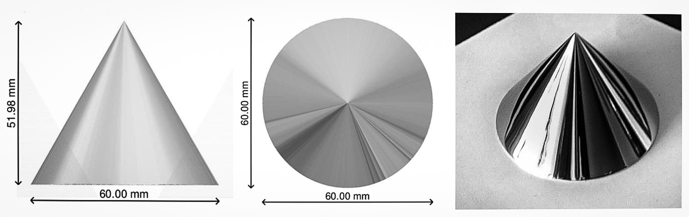
Looking at the above simulations and as demonstrated in my past Wolfram community contribution, reflection and anamorphism in a conical mirror result in considerable deformation of an image. It seems therefore unlikely that an image could be equal to its reflection in a conical mirror. I was therefore surprised reading the article "Self Anamorphic Images" by Andrew Crompton illustrating the existence of "self-anamorphic" images. "Self anamorphic" meaning: the image and its reflection are identical except for scaling and rotation. I wanted to investigate this further with Mathematica and constructed my own conical mirror to test this. A conical mirror is very sensitive to geometric precision and cannot be made accurately enough with reflecting foil as is the case for a cylindrical mirror. I needed to make a CNC precision turned cone, polished and subsequently chrome plated.
1. Geometry of reflection and anamorphism in a conical mirror
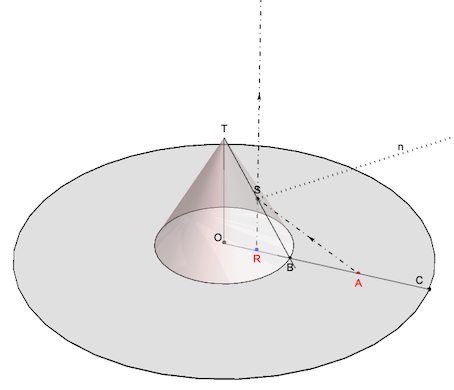
We first need another look at the geometry of reflection in a conical mirror: we take a cone with apex T, base radius 1 and opening angle 2alpha. Look down from an infinite viewpoint along the z-axis and we see a point A in the xy-plane reflected as a point R on the cone's base. Due to the radial symmetry of the cone, polar coordinates are the ideal choice. The polar coordinates of R are (r,t) and of A are (R,t). We can say that R is the reflection of A and A is the anamorphic image of R. A and R can be considered as an enantiomorphic point pair. According to the laws of reflection, in the triangles BRS and ARS, we can derive the relation: (1 - r) cot(alpha) == (R - r) cot(2 alpha). We solve this equation for r and R as follows (we standardize for a cone opening angle of alpha -> Pi/6):
eqn = (1 - r) Cot[alpha] == (R - r) Cot[2 alpha];
Solve[eqn, #] & /@ {R, r} // Flatten // Simplify
% /. alpha -> Pi/6 // Simplify
(*{R->1-(-1+r) Sec[2 alpha],r->1-(-1+R) Cos[2 alpha]}
{R->3-2 r,r->(3-R)/2}*)
We can now make the functions reflect and anamorph that convert the radial coordinates from R and A into one another. Since the points R and A are on the same line through the origin, their angular coordinate t remains unchanged.
reflect[r_] := (3 - r)/2
anamorph[r_] := 3 - 2 r
The functions reflect and anamorph are the inverse of one-another.
anamorph@reflect[2.75] == 2.75 (*True*)
2. Reflection of (filled) polar curves in a conical mirror
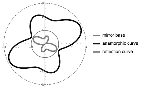
As curves can be interpreted as sets of points, we can also have enantiomorph curve-pairs. When expressed in polar coordinates, we apply the functions reflect or anamorph to the radial coordinates of each point in the curve. This is a simple curve and its reflection as seen looking down in a conical mirror:
butterfly[t_, a1_, a2_] := a1 - a2 Cos[t] Sin[3 t]
PolarPlot[{1, butterfly[t, 2, -1], reflect[butterfly[t, 2, -1]],
  3}, {t, -\[Pi], \[Pi]},
 PlotStyle -> {Gray, Directive[Black, AbsoluteThickness[4]],
   Directive[Gray, AbsoluteThickness[4]], Directive[Gray, DotDashed]},
  PlotLegends -> {"mirror rim", "anamorphic curve",
   "reflection curve", Nothing}]
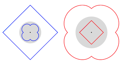
Regular polygons are interesting curves for reflection in a conical mirror. We see that reflect converts a square into a 4-petaled rose-like curve (left) and a 4-petaled rose-like curve into a square (right). The cone is represented by a gray disk in the center.
square[r_] := r Cos[Pi/4] Sec[2/4 ArcTan[Cot[2 t]]]
GraphicsRow[{Show[Graphics[{Point[{0, 0}], Opacity[.15], Disk[]}],
   PolarPlot[{square[2.5], reflect[square[1.75]]}, {t, -Pi, Pi},
    PlotStyle -> Blue]],
  Show[Graphics[{Point[{0, 0}], Opacity[.15], Disk[]}],
   PolarPlot[{square[.75], anamorph[square[.75]]}, {t, -Pi, Pi},
    PlotStyle -> Red]]}]
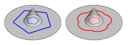
In 3D now, we can see below: (left) a pentagon reflects as a 5-petaled rose-like curve and (right) a 5-petaled rose-like curve reflects as a pentagon in a conical mirror. Or inversely: (left) the anamorphic image of a rose curve is a pentagon and (right) the anamorphic image of a pentagon is a rose curve using a conical mirror.
pentagon[r_] := r Cos[\[Pi]/5] Sec[2/5 ArcTan[Cot[(5 t)/2]]]
GraphicsRow[
 MapThread[
  Module[{alpha = Pi/6, op = .5, pts, ptsA, ptsR},
    pts = Table[{pentagon[#2], t}, {t, -3.141, 3.14, .01}];
    ptsR = (Flatten[{FromPolarCoordinates[#1], 0}] &) /@ pts;
    ptsA = Table[
      Flatten[{FromPolarCoordinates[{#1[pentagon[#2]], t}],
        0}], {t, -3.141, 3.14, .01}];
    Graphics3D[{{FaceForm[Lighter[LightGray, 1]],
       Cylinder[{{0, 0, 0}, {0, 0, -.01}}, 3]}, {Opacity[op],
       Cone[{{0, 0, 0}, {0, 0, 1/Tan[alpha]}}, 1]}, {#3,
       AbsoluteThickness[3], Line[ptsA]}, {#3, AbsoluteThickness[3],
       Line[ptsR]}}]] &, {{reflect, anamorph}, {2.1, .7}, {Blue,
    Red}}]]
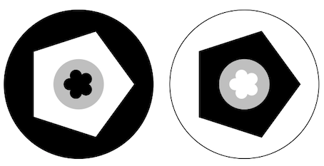
Using filled curves reveals an "optical illusion" with the apparent inversion of black and white: the white pentagon seems to reflect as a black rose and the black pentagon as a white rose?
filledPolarPlot[r_, edgeCol_, faceCol_] :=
 PolarPlot[r, {t, 0, 2 \[Pi]}, Axes -> False] /.
  Line[x__] :> {EdgeForm[edgeCol], FaceForm[faceCol], Polygon[x]}
GraphicsRow[MapThread[Show[filledPolarPlot[3, Black, #1],
    filledPolarPlot[pentagon[2.25], Black, #2],
    filledPolarPlot[1, Lighter[Gray, .5], Lighter[Gray, .5]],
    filledPolarPlot[reflect@pentagon[2.25], #3, #3]] &, {{Black,
    White}, {White, Black}, {Black, White}}]]
3. Condition for self anamorphism in a conical mirror
According to A. Crompton, Self Anamorphic Images, Journal of Mathematics and the ArtsPublication, June 2008: "A curve is called self-anamorphic if it has the same shape as its reflection in a curved mirror except for rotation and rescaling". We are looking for a periodic curve in polar coordinates in the x-y plane and centered around and reflected in an upright conical mirror. The radial coordinate R(t) of the curve should have a period of 2 Pi and can be represented by its Fourier series approximation:
R[t] = Sum[
  an Cos[n t] + bn Sin[n t], {n, 0,
   7}] (*limit of 8 terms sufficient for the discussion here*)
As stated at the beginning, to be self - anamorphic, the reflected curve r(t) needs to be a scaled and rotated version of R(t) and a linear combination of R(t) a +b R(t+t0) . If the scaling factor is m and the rotation angle t0, we can write the equations:
eqns = TrigExpand //@ (a + b (Cos[n t] an + Sin[n t] bn) ==
    m (Cos[n (t + t0)] an + Sin[n (t + t0)] bn))
(*a+an b Cos[n t]+b bn Sin[n t]== an m Cos[n t] Cos[n t0]+bn m Cos[n \
t0] Sin[n t]+bn m Cos[n t] Sin[n t0]-an m Sin[n t] Sin[n t0]*)
\
Solve[eqns, {an, bn}]
(*{an->(a+b Sin[n t] bn-m Sin[n (t+t0)] bi)/(b Cos[n t]+m Cos[n \
(t+t0)])}
{bn->(a-b Cos[n t] an-m Cos[n (t+t0)] an)/(b Sin[n t]+m Sin[n \
(t+t0)])}*)
We have now two equations with as coefficient matrix:
mat = {{b/m + Cos[n t0], Sin[n t0]}, {-Sin[n t0], b/m + Cos[n t0]}}
(*{{b/m+Cos[n t0],Sin[n t0]},{-Sin[n t0],b/m+Cos[n t0]}}*)
To have (an indefinite number of) solutions, we need the determinant of the coefficient matrix to be zero.
det = Det[mat] // FullSimplify // Apart
(*( b^2+m^2)/m^2+(2 b Cos[n t0])/m*)
FindInstance[
 det == 0, {m, b, Cos[n t0]}]
(*{{m->1,b\[Rule]1,Cos[n t0]->-1}}*)
Flatten@
 Solve[Cos[(nt0)] == -1, (nt0)]
(* nt0->ConditionalExpression[-Pi+2 Pi \
c1,Element[c1,Integers]],nt0->ConditionalExpression[Pi+2 Pi \
c1,Element[c1,Integers]] *)
For Cos(n t0) to be -1, possible combinations of t0 and (n t0) must be odd integer multiples of Pi . This gives a table of the possible combinations of frequency indices n and rotations t0 that will produce self-anamorphic curves. t0 is the rotation angle between the curve and its reflection and n is the frequency index of the coefficient of the Fourier expansion of the curve:
Grid[lst =
  Prepend[Cases[
    Table[Flatten[{t0,
       Table[180 \[Degree]/t0 (2 p + 1), {p, 0, 6}]}], {t0,
      10 \[Degree], 360 \[Degree], 1 \[Degree]}], {_?NumericQ, _?
      IntegerQ, ___}],
   Style[#, 15] & /@ {t0, n1, n2, n3, n4, n5, n6, n7}],
 Background -> {{LightGray}, {LightGray}}]
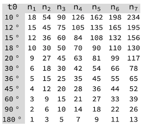
We can conclude that we have an infinite amount of self-anamorphic curves by reflection in a conical mirror. Curves represented by Fourier series can have any values of the a and b coefficients provided that n*t0 is an odd multiple of Pi. The above table gives the values of n needed for each rotation t0 between the curve and its reflection.
4. Examples of self anamorphism in a conical mirror.
The curve that will reflect as a scaled copy of itself, rotated over 90 degree can be approximately represented by an expansion of the form a0+a1 cos(2t)+a2 cos(6t)+a3 cos(10t)+a4cos(14t)+a5 cos(18t)+... The ai can be any combination that keeps the curve within the limits of reflection by the cone. (this is for an opening angle of 30 degrees, the annulus((0,0),(1,3))). here is one example out of an infinite many:
With[{a1 = 0.189, a2 = -0.08, a3 = 0.048, a4 = 0},
 Module[{polaR},
  polaR = 1.5` + a1 Cos[2 t] + a2 Cos[6 t] + a3 Cos[10 t] +
    a4 Cos[14 t];
  Show[filledPolarPlot[polaR, Thick, White],
   Graphics[{Circle[], LightGray, Disk[]}],
   filledPolarPlot[reflect[polaR], Thick, White],
   Graphics[Circle[{0, 0}, .01]], Background -> LightGray]]]
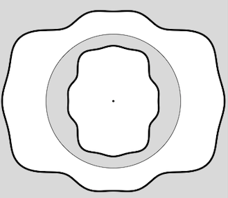
This animation shows the shape variations if we change only the coefficient a1. All these intermediate curves are self-anamorphic with their reflections in a conical mirror.
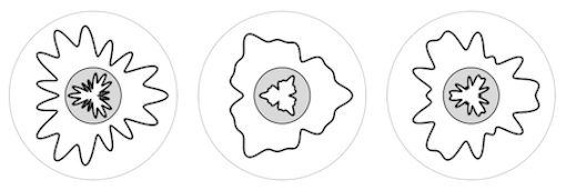
This is a set of 3 curves with t0=60 degree:
GraphicsRow@
 MapThread[
  Module[{polaR},
    polaR = 1.95 + #1 Cos[3 t] + #2 Cos[9 t] + #3 Cos[15 t];
    Show[filledPolarPlot[3, Thin, White],
     filledPolarPlot[polaR, Thick, White],
     filledPolarPlot[1, Black, LightGray],
     filledPolarPlot[reflect[polaR], Thick,
      White]]] &, {{.35, .3, .34}, {-.035, .164, .238}, {.4, .09, \
-.222}}]
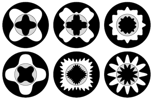
... and 6 self anamorphic curves rotated over 45 degree:(here, we use filled curves and one can observe again the apparent black-white inversion between the white curves and their black reflections. As was demonstrated before, this inversion is merely an optical illusion.
Grid@Partition[
  MapThread[
   Module[{polaR},
     polaR = 1.5 + #1 Cos[4 t] + #2 Cos[12 t] + #3 Cos[20 t] + #4 Cos[
         28 t]; Show[filledPolarPlot[2.1, Black, Black],
      filledPolarPlot[polaR, Black, White],
      filledPolarPlot[1, Black, LightGray],
      filledPolarPlot[
       reflect[1.5 + #1 Cos[4 t] + #2 Cos[12 t] + #3 Cos[
           20 t] + #4 Cos[28 t]], Black,
       Black]]] &, {{-0.424`, -0.424`, -0.003`,
     0.4`, -0.219`, -0.074`}, {0.008`, 0.128`, 0.127`, -0.037`, 0,
     0.377`}, {0.002`, 0.002`, 0.053`, 0.`, 0, 0}, {0.001`, 0.001`,
     0.001`, 0, 0.143`, 0.03`}}], 3]
This GIF shows a test to check if the curves are self-anamorphic i.e. the curves and their reflections are equal except for rotation and scaling. The video shows a 45 degree curve (bleu) of the form 1.5+a0.4 Cos[4t]-.137 Cos[12t]+a3Cos[20t] (n values per previous table) and its reflection (red). We first rotate the reflected curve up to 45 degrees and scale it up to coincide with the red original. Both are equal and, even if we change e.g the a3 coefficient at the end of the video, both shapes stay identical.
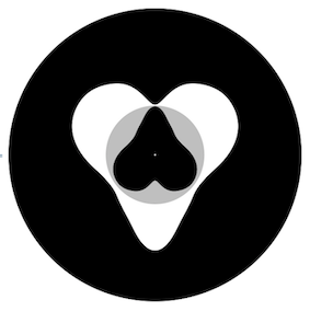
4. The remarkable Heart Curve.
An exceptional curve was found by Andrew Crompton in the above mentioned article: a certain combination of the 180 degree coefficients produces a heart-like curve which is quite remarkable. I am repeating his calculations here...
Module[{heart, a1 = -0.1061`, a2 = -.3806, a3 = 0.0843`,
  a4 = -0.0552`, a5 = 0.028`, a6 = -0.0165`, a7 = 0.0068`},
 heart[aa_] :=
  1.5` + a1 Cos[t] - aa Cos[3 t] + a3 Cos[5 t] - a4 Cos[7 t] +
   a5 Cos[9 t] - a6 Cos[11 t] + a7 Cos[13 t];
 Rotate[Show[{Graphics[{Disk[{0, 0}, 3]}],
    filledPolarPlot[heart[a2], Black, White],
    Graphics[{Lighter[Gray, .5], Circle[], Disk[]}],
    filledPolarPlot[reflect[heart[a2]], Black, Black],
    Graphics[{EdgeForm[Black], FaceForm[White], Disk[{0, 0}, .025]}]},
    Axes -> False, PlotRange -> 3], 3 Pi/2]]
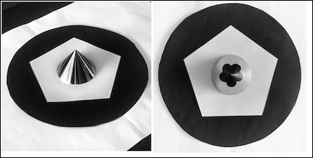
... and show the result as reflected it in my conical mirror.
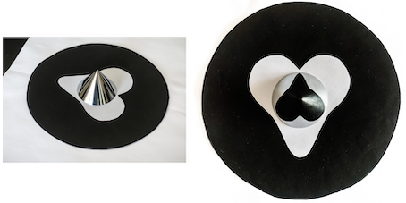
If we do the same in two colors, as in the following photo, we can easily see why the apparent black-white inversion above was an optical illusion:
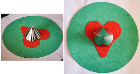
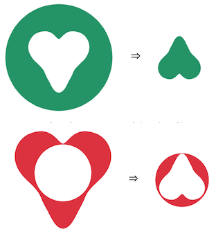
The following illustration shows how it is not the green heart that reflects as the red heart but it is the green ring that becomes the green heart and the red ring that reflects as the red heart! This can easily be observed in two colors but it creates optical confusion when in black and white.
Module[{heart, a1 = -0.1061`, a2 = -.3806, a3 = 0.0843`,
  a4 = -0.0552`, a5 = 0.028`, a6 = -0.0165`, a7 = 0.0068`,
  green = RGBColor[12/256, 150/256, 100/256],
  red = RGBColor[225/256, 45/256, 52/256]},
 polaR = 1.5` + a1 Cos[t] - a2 Cos[3 t] + a3 Cos[5 t] - a4 Cos[7 t] +
   a5 Cos[9 t] - a6 Cos[11 t] + a7 Cos[13 t];
 Column[{Row[{Rotate[Show[filledPolarPlot[3., green, green],
       filledPolarPlot[polaR, White, White]], 3 Pi/2],
     Style["  \[DoubleRightArrow]  ", 26],
     Rotate[Show[filledPolarPlot[reflect@polaR, green, green],
       ImageSize -> 50], 3 Pi/2]}],
   Row[{Rotate[Show[
       filledPolarPlot[polaR, red, red],
       filledPolarPlot[1, White, White], ImageSize -> 200], 3 Pi/2],
     Style["  \[DoubleRightArrow]  ", 26],
     Rotate[Show[filledPolarPlot[1, red, red],
       filledPolarPlot[reflect@polaR, White, White]], 3 Pi/2]}]}]]
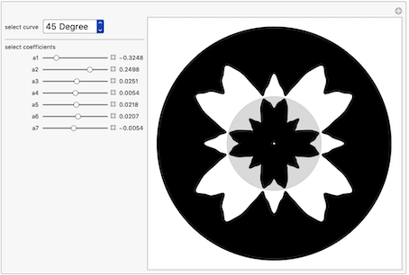
To conclude, here is a Manipulate that can be used to explore the infinite amount of self-anamorphic curves. Select the rotation angle between the curve and its reflection, then set the 7 coefficients of the curves Fourier expansion and see the resulting curve and it, self-anamorphic reflection. Maybe you can find another recognizable or exceptional curve among the millions? Good luck and have fun!
Manipulate[
 Module[{lst, curves, polaR},
  lst = Cases[
    Table[Flatten[{t0,
       Table[180 Degree/t0 (2 p + 1), {p, 0, 6}]}], {t0, 10 Degree,
      360 Degree, 1 Degree}], {_?NumericQ, _?IntegerQ, ___}];
  curves = MapThread[
    1.5 + a1 Cos[#1 t] + a2 Cos[#2 t] + a3 Cos[#3 t] + a4 Cos[#4 t] +
      a5 Cos[#5 t] + a6 Cos[#6 t] + a7 Cos[#7 t] &,
    Transpose[Rest /@ lst]]; polaR = curves[[sc]];
  Rotate[Show[{Graphics[{Disk[{0, 0}, 2.5]}],
     filledPolarPlot[polaR, Black, White],
     Graphics[{Lighter[Gray, .5], Circle[], LightGray, Disk[]}],
     filledPolarPlot[reflect[polaR], Black, Black],
     Graphics[{EdgeForm[Black], FaceForm[White],
       Disk[{0, 0}, .025]}]}, Axes -> False, PlotRange -> 2.5],
   3 Pi/2]],
 {{sc, 11, "select curve"},
  Rule @@@ Transpose@{Range[1, 11],
     ToString /@ (First /@ lst)}}, Delimiter, "select coefficients",
 {{a1, -0.1061}, -.5, .5, .0001, ImageSize -> Small,
  Appearance -> "Labeled"},
 {{a2, .3806}, -.5, .5, .0001, ImageSize -> Small,
  Appearance -> "Labeled"}, {{a3, .0843}, -.5, .5, .0001,
  ImageSize -> Small, Appearance -> "Labeled"},
 {{a4, 0.0552}, -.5, .5, .0001, ImageSize -> Small,
  Appearance -> "Labeled"},
 {{a5, .028}, -.5, .5, .0001, ImageSize -> Small,
  Appearance -> "Labeled"},
 {{a6, .0165}, -.2, .2, .0001, ImageSize -> Small,
  Appearance -> "Labeled"}, {{a7, .0068}, -.1, .1, .0001,
  ImageSize -> Small, Appearance -> "Labeled"}]