Message Boards Message Boards

0
|
12983 Views
|
10 Replies
|
7 Total Likes
View groups...
Share
Share this post:

How do you make a phase line

How do you make a "phase line" showing the stable and unstable points and the arrows? 
Thanks
Jake
POSTED BY: Jake Trexel
10 Replies
BTW, 

the flow shown on the line in the post by Jake for f=x^2 is incorrect. It seems to show an unstable fixed point at x=1. The flow that corresponds to D[x,t]=x^2 has only one fixed point at x=0. That fixed point is "semistable". 

The code in my post below will not work for f=x^2. This one will:
 zeros = DeleteDuplicates[NSolve[f[x] == 0, x, Reals]];
 M = 12.; If[Length[zeros] == 0, Print["There are no zeros."],
  If[(Min[x /. zeros] - Max[x /. zeros]) != 0,
   Show[Join[{Graphics[
       Line[{{Min[x /. zeros] -
           0.2 (Abs[Abs[Max[x /. zeros]] - Min[x /. zeros]]),
          0}, {Max[x /. zeros] +
           0.2 (Abs[Abs[Max[x /. zeros]] - Min[x /. zeros]]), 0}}]]},
     Table[Graphics[{Disk[{x /. zeros[[k]], 0}, 0.1],
       Text[Style[x /. zeros[[k]], Medium], {x /. zeros[[k]],
         0.4}]}], {k, 1, Length[zeros]}],
    Table[Graphics[{Thick, {Arrowheads[Medium],
        Arrow[{{Min[x /. zeros[[1]]] -
            0.2 (Abs[Abs[Max[x /. zeros]] - Min[x /. zeros]]) +
            k/M (Abs[Abs[Max[x /. zeros]] - Min[x /. zeros]]),
           0}, {Min[x /. zeros] -
            0.2 (Abs[
               Abs[Max[x /. zeros]] - Min[x /. zeros]]) + (k +
                0.01 f[Min[x /. zeros] -
                   0.2 (Abs[Abs[Max[x /. zeros]] - Min[x /. zeros]]) +
                    k/M (Abs[
                    Abs[Max[x /. zeros]] - Min[x /. zeros]])])/
              M (Abs[Abs[Max[x /. zeros]] - Min[x /. zeros]]),
           0}}]}}], {k, 0, M + Floor[0.4*M]}]], ImageSize -> Large],
  Show[Join[{Graphics[
      Line[{{(x /. zeros[[1]]) - 1, 0}, {(x /. zeros[[1]]) + 1,
         0}}]]}, {Graphics[{Disk[{x /. zeros[[1]], 0}, 0.04],
       Text[Style[x /. zeros[[1]], Medium], {x /. zeros[[1]],
         0.4}]}]},
    Table[Graphics[{Thick, {Arrowheads[Medium],
        Arrow[{{(x /. zeros[[1]]) - 1. + k/M *2.,
           0}, {(x /. zeros[[1]]) -
            1 + (k + 0.01 f[(x /. zeros[[1]]) - 1. + 2.*k/M ])/M *2.,
           0}}]}}], {k, 0, M}]]]]]
 For 
f[x_] := x^2

this gives the correct flow


M.
POSTED BY: Marco Thiel
How about StreamPlot?
StreamPlot[{x - 1, 0}, {x, 0, 2}, {y, 0, 1}]
or brute force?

Graphics[
Table[
  Arrow[If[
    x < 1, {{x, 0}, {x - 0.2, 0}}, {{x, 0}, {x + 0.2, 0}}]], {x, 0,
   2, .2}]
]
POSTED BY: W. Craig Carter
Hi,

this is probably overkill, but well, it produces something close to what you want, I guess...

I used a different function to show a more interesting case.
f[x_] := -1.3 x^2 + 0.2 x^3 + 2

This function looks like this:


The program is a bit longer than the one given above, but still quite straight forward..
 (*First get the fixed points of the flow*)
 zeros = NSolve[f[x] == 0, x];
 
 (*Determine rough number of arrows; the program adds some arrows at the beginning and the end*)
 M = 12.;
 Show[
 (*base coordinate line*)
 
  Join[{Graphics[
    Line[{{Min[x /. zeros] -
        0.2 (Abs[Abs[Max[x /. zeros]] - Min[x /. zeros]]),
       0}, {Max[x /. zeros] +
        0.2 (Abs[Abs[Max[x /. zeros]] - Min[x /. zeros]]), 0}}]]},

(*mark the fixed points and label them*)
  Table[Graphics[{Disk[{x /. zeros[[k]], 0}, 0.1],
     Text[Style[x /. zeros[[k]], Medium], {x /. zeros[[k]],
       0.4}]}], {k, 1, Length[zeros]}],

(*draw the arrows*)
  Table[Graphics[{Thick, {Arrowheads[Medium],
      Arrow[{{Min[x /. zeros] -
          0.2 (Abs[Abs[Max[x /. zeros]] - Min[x /. zeros]]) +
          k/M (Abs[Abs[Max[x /. zeros]] - Min[x /. zeros]]),
         0}, {Min[x /. zeros] -
          0.2 (Abs[
             Abs[Max[x /. zeros]] - Min[x /. zeros]]) + (k +
              0.01 f[Min[x /. zeros] -
                 0.2 (Abs[Abs[Max[x /. zeros]] - Min[x /. zeros]]) +
                 k/M (Abs[Abs[Max[x /. zeros]] - Min[x /. zeros]])])/
            M (Abs[Abs[Max[x /. zeros]] - Min[x /. zeros]]),
         0}}]}}], {k, 0, M + Floor[0.4*M]}]], ImageSize -> Large]
This is the output:


It's in a very basic form and should be cleaned up, but does the trick.

Cheers,
M.
POSTED BY: Marco Thiel
Here's the solution with streamplot. We need to enter the functions in a slightly different way now:
 f = {x^2 - 0.2 x^3 - 2, 0}
 
 or
 
 f = {-1.3 x^2 + 0.2 x^3 + 2, 0}
 
 or
 
 f = {x^2, 0}

So we only need to add a second component which is zero. The program distinguishes again between the three main cases.

 M = 12; zeros = DeleteDuplicates[NSolve[f[[1]] == 0, x, Reals]];
 
 
 If[Length[zeros] == 0,
 
  (*no fixed points*)
  Print["There are no zeros."],
 
  If[(Min[x /. zeros] - Max[x /. zeros]) != 0,
  (*more than one fixed point*)
 
  StreamPlot[
   f, {x, Min[x /. zeros] - 0.2*(Max[x /. zeros] - Min[x /. zeros]),
    Max[x /. zeros] +
     0.2*(Max[x /. zeros] - Min[x /. zeros])}, {y, -0.1, 0.1},
   AspectRatio -> 0.1, ImageSize -> Large, Frame -> None,
   StreamPoints -> {Table[{x,
       0}, {{x,
        Min[x /. zeros] - 0.2*(Max[x /. zeros] - Min[x /. zeros]),
        Max[x /. zeros] +
         0.2*(Max[x /. zeros] - Min[x /. zeros]), (Max[x /. zeros] -
           Min[x /. zeros])/M}}]},
   Epilog ->
    Table[{{Red, Disk[{x /. zeros[[i]], 0.}, {0.1, 0.05}]},
      Text[Style[x /. zeros[[i]], Medium], {x /. zeros[[i]],
        0.15}]}, {i, 1, Length[zeros]}]],
 
  (*xeactly one fixed point*)
 
  StreamPlot[
   f, {x, (x /. zeros[[1]]) - 1., (x /. zeros[[1]]) + 1.}, {y, -0.05,
    0.05}, AspectRatio -> 0.1, ImageSize -> Large, Frame -> None,
   StreamPoints -> {Table[{x,
       0}, {{x, (x /. zeros[[1]]) - 1., (x /. zeros[[1]]) + 1.,
        2./M}}]},
   Epilog ->
    Table[{{Red, Disk[{x /. zeros[[i]], 0.}, {0.04, 0.03}]},
      Text[Style[x /. zeros[[i]], Medium], {x /. zeros[[i]],
        0.06}]}, {i, 1, Length[zeros]}]]]]

The problem is that in that version we have to adapt the plot range on the y-axis and also slighty change the size of the red dots every time we run it. It is easy to fix, but the code should show the idea. A typical output figure looks like this:
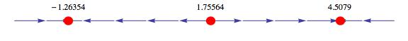


M.
POSTED BY: Marco Thiel
Attached is another variant to the many solutions above. Thank you for allowing me to share.
 (* PROGRAM BEGINS *)
 
 (* Clear memory *)
 Clear["Global`*"];
 
 (* Enter a trial (polynomial) function with real roots. *)
 f[x_] := (0)x^5 + (0)x^4 + (0)x^3 + (-1)x^2 + (0)x + (0)1 ;
 
 (* Find roots *)
roots = N[ x /. Solve[ f[x]==0,x]];

(* Assign phase lines to various conditions *)
test = Which[
f[-1] < 0 && f[1] < 0, "\[LeftArrow] \[EmptyDownTriangle] \[LeftArrow]",
f[-1] < 0 && f[1] > 0, "\[LeftArrow] \[EmptyDownTriangle] ->",
f[-1] > 0 && f[1] < 0, "-> \[FilledCircle] \[LeftArrow]",
f[-1] > 0 && f[1] > 0, "-> \[EmptyDownTriangle] ->"];

(* Assign markers to the roots, based on the sign of the
function derivative at the root location. *)
marker = ((D[f[x],x] /. x -> roots) // Sign )/.
{ 1 -> "\[LeftArrow] \[EmptyCircle] ->", -1 -> "-> \[FilledCircle] \[LeftArrow]", 0 -> test};
(* Generate plots *)
Which[ roots == Re[roots],
{
(* Generate plot limits based on the roots. *)
xmin = 2 Min[-1, Min[roots]];
xmax = 2 Max[1 , Max[roots]];
ylim = f[#]& /@ Max[x /.  Solve[ D[f[x],x] == 0, x]];
(* When the roots are real,...*)
(* Generate f (t)-t plot. *)
plt = Plot[ f[x], {x, xmin, xmax},
ImageSize -> 100];
(* Generate phase plot. *)
phs = ListPlot[ {Thread[{roots,0}][[#]]},
PlotMarkers -> If[Length[marker]!=0, {marker[[#]]} , "x"]
(* Close ListPlot *)]& /@ Table[i,{i,1,Length[roots]}];

(* Combine phase and f (t)-t plots. *)
Show[ {plt (* Delete plt if original plot is not desired *), phs},
AxesLabel  -> {"x", "y"},
PlotLabel  -> Style["Phase Plot", 24],
LabelStyle -> 24,
PlotRange  -> { {xmin, xmax}, {-2ylim, 2ylim} },
Epilog     -> Inset[(* Begin Framed *)Framed[Style[StringJoin["Roots = ",ToString[roots]], 24,
             Background -> White(* End Framed *)]],
             Scaled[{0.5,0.15}]],
ImageSize  -> 500]},

(* When the roots are imaginary,...*)
roots !=  Re[roots], {Print["Complex roots encountered.
There are no fixed points. Phase plot is not generated."]}(* Close Which *)][[1]]
(* PROGRAM ENDS *)
POSTED BY: Isaac Abraham
Dear Jake,

no worries. The code only appears long because of the three cases (no fixed point, one fixed point or more). It is basically only a plotting issue. I am sure that it is quite possible to shorten the code substantially. For example this bit
Abs[Abs[Max[x /. zeros]] - Min[x /. zeros]]
comes up over and over again. One could just define it once and then use it in the remainder of the code. I did not mean to write short code here, just to illustrate the idea. Isaac's "Which"-command makes the code shorter as well. The epilog function could be defined once and reused later in the code as well. 

Actually, one should improve this a bit and then write it as a function, the definition of which could go into the initialisation of the notebook or into a package.

Cheers,
M.
POSTED BY: Marco Thiel
http://reference.wolfram.com/mathematica/ref/VectorPlot.html<br>
POSTED BY: Frank Kampas
Thanks.  I am fine with solving the problem, what I dont know how to make with Mathematic is what I am showing in the picture.  Hope this explains my problem better.
POSTED BY: Jake Trexel
The second solution is closer but I am still missing the dots and numbers.  Is there a way to add them?  I know it is simple to do by hand.  Would you recommend using a drawing program to make it and add it as a picture?  I am needing this for a text book on dynamic systems that I am writing.   That's why it is really important to have all of the parts.  I would really like to have a closed circle and an open circle to show the unstable and stable points.  
Thanks
POSTED BY: Jake Trexel
Thanks so much for all the work you did.  I never expected the code to be so long. 
Jake
POSTED BY: Jake Trexel
Reply to this discussion
Community posts can be styled and formatted using the Markdown syntax.
Reply Preview
Attachments
Remove
or Discard

Group Abstract Group Abstract