Purpose and Methods:
Some time ago I published on the WFR (Wolfram Function Repository) the function MusicalScaleSample, where a sound scale sample can be generated. Which can be 30 different scales possible with this WFR item. But how to know which scale was the origin that generated the samples themselves? This is what this work is about, where I approach some methods, from semi-mechanics to machine learning with the comment on the results afterwards.
The methods covered here have this order below (of course, there are many other methods, here some in a briefly addressed way and others more detailed):
Semi-mechanical / Pitch Frequency
Pitch Sound Note
Classify / Method Neural Net
Classify / Method Naive Bayes
Customized ResNet
These methods are (more or less) in the order of machine complexity x efficiency, the latter, Customized ResNet, was the method that generated the best results (as we going to see). In the course of this work I will comment on each method, it´s limitations and results.
Initial Samples / Sound:
The musical scales follow patterns that can be represented by the distances between your notes, so, as a first step, we have these distances below:
sequences = {"MajorPentatonic" -> {0, 2, 2, 3, 2},
   "MinorPentatonic" -> {0, 3, 2, 2, 3},
   "NeopolitanMajor" -> {0, 1, 2, 2, 2, 2, 2},
   "NeopolitanMinor" -> {0, 1, 2, 2, 2, 1, 3},
   "HungarianMajor" -> {0, 3, 1, 2, 1, 2, 1},
   "HungarianMinor" -> {0, 2, 1, 3, 1, 1, 3},
   "HungarianGypsy" -> {0, 2, 2, 2, 1, 1, 2},
   "HarmonicMajor" -> {0, 2, 2, 1, 2, 1, 3},
   "HarmonicMinor" -> {0, 2, 1, 2, 2, 1, 3},
   "DoubleHarmonic" -> {0, 1, 3, 1, 2, 1, 3},
   "JazzMinor" -> {0, 2, 1, 2, 2, 2, 2},
   "Overtone" -> {0, 2, 2, 2, 1, 2, 1},
   "BluesScale" -> {0, 3, 2, 1, 1, 3},
   "Chromatic" -> {0, 1, 1, 1, 1, 1, 1, 1, 1, 1, 1, 1},
   "WholeTone" -> {0, 2, 2, 2, 2, 2},
   "DiminishedWholeTone" -> {0, 1, 2, 1, 2, 2, 2},
   "Symmetrical" -> {0, 1, 2, 1, 2, 1, 2, 1},
   "Arabian" -> {0, 2, 2, 1, 1, 2, 2}, "Balinese" -> {0, 1, 2, 4, 1},
   "Byzantine" -> {0, 1, 3, 1, 2, 1, 3},
   "Persian" -> {0, 1, 3, 1, 1, 2, 3},
   "EastIndianPurvi" -> {0, 1, 3, 2, 1, 1, 3},
   "Oriental" -> {0, 1, 3, 1, 1, 3, 1},
   "GagakuRyoSenPou" -> {0, 2, 2, 3, 2},
   "Zokugaku" -> {0, 3, 2, 2, 3}, "InSenPou" -> {0, 1, 4, 2, 1},
   "Okinawa" -> {0, 4, 1, 2, 4}, "Enigmatic" -> {0, 1, 3, 2, 2, 2, 1},
    "EightToneSpanish" -> {0, 1, 2, 1, 1, 1, 2, 2},
   "Prometheus" -> {0, 2, 2, 2, 3, 1}};
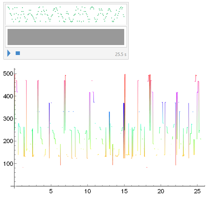
Below, is a sample of a scale, in this case "Enigmatic", as well as its signature through the PitchRecognize command represented in a ListLinePlot chart. It is worth noting that the duration of each note is relatively short, so that the peaks of the notes do not extend like a hill, but rather more defined peaks so that there are better chances of being recognized:
Sound@Table[
  ResourceFunction["MusicalScaleSample"]["Enigmatic", "Tone" -> "C3",
   "NoteInterval" -> 0.15, "Playing" -> "Mechanical"], 5]
ListLinePlot[PitchRecognize[%],
 ColorFunction -> Function[{x, y}, Hue[y]], PlotStyle -> Thin,
 AxesStyle -> Directive[Black, 12]]
Semi-mechanical / Pitch Frequency
First, a function is developed that generates the musical note through PitchRecognize/Frequency; the equation itself is mechanical, although the recognition command already has characteristics of neural networks associated:
notes[x_] :=
 Keys@Counts[
   Round[-36 + (12 Log[1/55 2^(3/4) #])/Log[2]] & /@
    QuantityMagnitude@
     DeleteMissing@Values@PitchRecognize[x, "Frequency"]]
Below is the conversion of the intervals of the notes in the notes themselves (taking into account 7 different octaves):
numb = Table[-48 + # & /@
     Flatten[# + Accumulate[Values@sequences[[x]]] & /@ {0, 12, 24,
        36, 48, 60, 72}] -> Keys[sequences[[x]]], {x, 1, 30}];
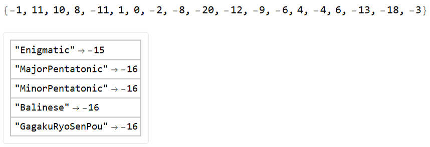
Testing the first method with a “Enigmatic” class scale sample, where we will get the musical notes and the prediction in the results. The result gives values and weights for both notes found and anti-values for notes not found on the scale. The result is this:
Table[Values@numb[[i]] ->
   Subtract[Values[Counts[MemberQ[Keys@numb[[i]], #] & /@ test]][[1]],
     Values[Counts[MemberQ[test, #] & /@ Keys@numb[[i]]]][[1]]], {i,
   1, 30}] // Dataset[MaximalBy[#, Values, 5]] &
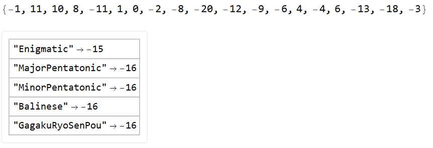
Note that in the case above the scale was correctly identified, but this method is very fragile and for most scales and attempts the result is quite unsatisfactory.
Pitch Sound Note
This next method relies more on the ability to recognize of the PitchRecognize command to recognize the frequencies, compared to the first method. The result is also given in valued scores and a prediction of which scale was used (in this case, a “Enigmatic” sample was also used):
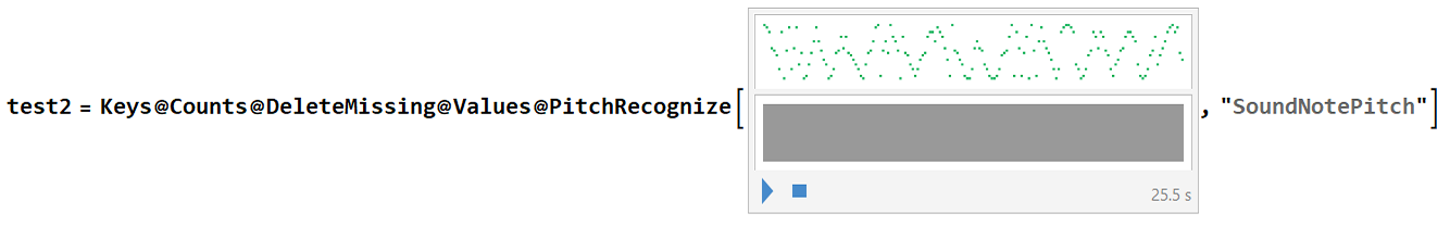
Table[Values@numb[[i]] ->
   Subtract[
    Values[Counts[MemberQ[Keys@numb[[i]], #] & /@ test2]][[1]],
    Values[Counts[MemberQ[test2, #] & /@ Keys@numb[[i]]]][[1]]], {i,
   1, 30}] // Dataset[MaximalBy[#, Values, 5]] &
Realize that the result was identical between the first two methods discussed, at least for the musical scale “Enigmatic” sample given. Normally, this method is also not very reliable and most of the time (with most musical scales) is wrong, which was tested, although in this case above I got it right.
Classify / Method Neural Net
We will use a Neural Net classification method in this next attempt, to see if by this specific method the result is more satisfactory when working with Audio. First, we will generate a total of 50 samples of each type of musical scale class. Each sample in this case is 25.5 seconds in size formed with 5 random reproductions sequence by the specific scale. The tone will be maintained in all tests in “C3” with two octaves (default) and the playing method will always be mechanical for each note to have the same exact duration:
n = 50; samp1 =
 RandomSample@
  Flatten@Table[(Sound@
         Table[ResourceFunction["MusicalScaleSample"][#,
           "Tone" -> "C3", "NoteInterval" -> 0.15,
           "Playing" -> "Mechanical"], 5] -> #) & /@ Keys@sequences,
    n];
Above, “samp1” was generated with 1500 samples, then changed to “stest1” with 300 samples to test the result of the classifiers. Now we can use Classify, as well as test it for the result and accuracy of the method:
c2 = Classify[samp1, Method -> "NeuralNetwork"]
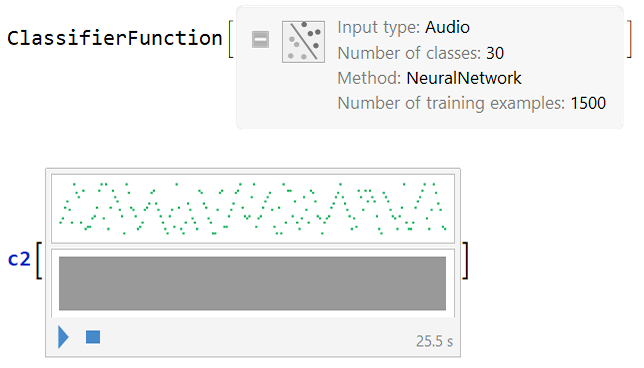
ClassifierMeasurements[c2, stest1, "Accuracy"]
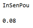
As we can observe above, this method is far from being the best method to predict which musical scale in the case, it only gave a value of 8% accuracy!
Classify / Method Naive Bayes
This next method is another option for the Classify function, an option that usually works best with Audio. Below we will see the result of the classifier with its prediction and accuracy:
c3 = Classify[samp1, Method -> "NaiveBayes"]
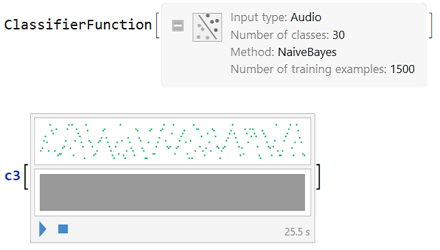
ClassifierMeasurements[c3, stest1, "Accuracy"]
We see that by this method above (Naive Bayes), the result was already better to predict the original musical scale used, although it is still far from ideal, especially for some of the musical scales classes.
Customized ResNet
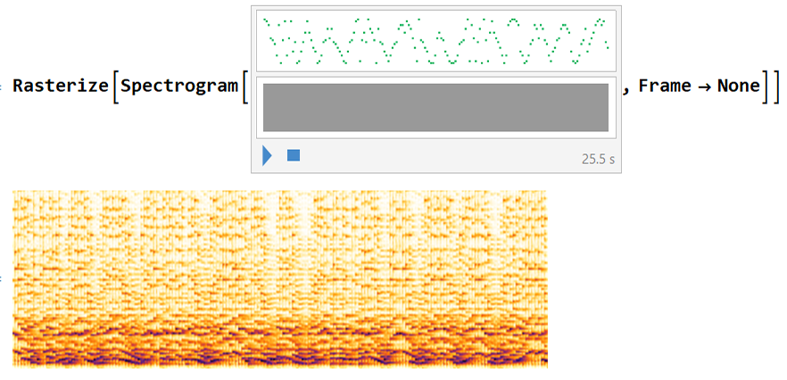
The last method I tested in this work is by far the best method. First big difference is the transformation (Fourier) of Audio to its spectrum, since the classification of images proved to be a more powerful tool in this case. Below is an example of an Audio sample and its corresponding image to be classified by Machine Learning process:
In order to generate the samples to be performed in the machine learning, some small modifications were made:
Instead of 5 reproductions followed by the scale in each sample, 10 reproductions were made, because more reproductions, it becomes clearer which is the identity of the scale.
A slightly higher value of the note interval was also used to make it easier to identify the sound of each note, this value was adapted together with the reproductions followed, so that, each sample has an exact 60 seconds of duration.
Another change was to directly specify the RasterSize and ImageSize for each sample to have a slightly better definition.
Below, 100 samples of each scale class were generated, totaling 3000 samples (the time for this process was approximately 3 hours and the sample set size was just over 1GB):
n = 100; samp =
 RandomSample@
  Flatten@Table[(Rasterize[
         Spectrogram[
          Sound@Table[
            ResourceFunction["MusicalScaleSample"][#, "Tone" -> "C3",
             "NoteInterval" -> 0.17646, "Playing" -> "Mechanical"],
            10], Frame -> None], RasterSize -> 600,
         ImageSize -> 300] -> #) & /@ Keys@sequences, n];
The generator above was used also for a set: "stest" with 30 samples from each class totaling 900 total samples and a smaller set "stest2" of 15 samples from each class totaling 450 total samples.
To better store these sample sets above I used DumpSave and the .MX file format:
filepath2 = FileNameJoin[{NotebookDirectory[], "samp.mx"}];
DumpSave[filepath2, {samp}];
filepath3 = FileNameJoin[{NotebookDirectory[], "stest.mx"}];
DumpSave[filepath3, {stest}];
filepath4 = FileNameJoin[{NotebookDirectory[], "stest2.mx"}];
DumpSave[filepath4, {stest2}];
Quit[]
We can retrieve the sets with the simple Get command:
SetDirectory[NotebookDirectory[]];
Get["samp.mx"]
Get["stest.mx"]
Get["stest2.mx"]
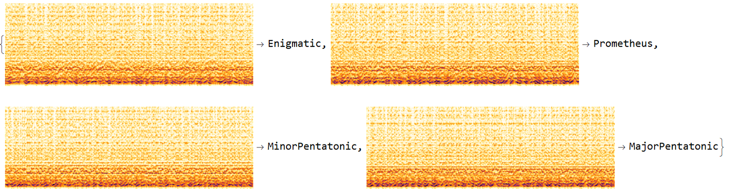
Example of how the main set contains the samples and their definitions:
samp[[5 ;; 8]]
We will now start to develop the customized NetChain. First, we create a directory for the classifier batches:
dirModel = CreateDirectory[];
Than, we downloaded the ResNet, which in this case I used the ResNet-152 from Wolfram Neural Repository, but we discarded the last 3 layers in order to be able to customize the output and some characteristics of behavior:
tempNet =
 Take[NetModel[
   "ResNet-152 Trained on ImageNet Competition Data"], {1, -4}]
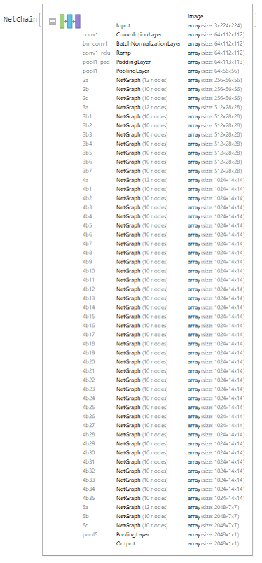
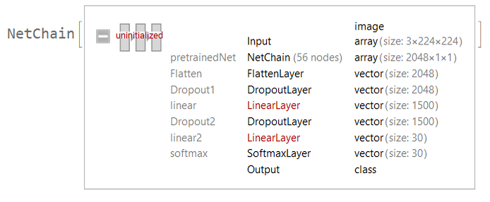
We added some layers to increase the complexity and so that it can learn new features. Just as we defined, the 30 different classes of different musical scales to be used by the neural network:
newNet = NetChain[<|"pretrainedNet" -> tempNet,
   "Flatten" -> FlattenLayer[], "Dropout1" -> DropoutLayer[0.2],
   "linear" -> LinearLayer[1500], "Dropout2" -> DropoutLayer[0.2],
   "linear2" -> LinearLayer[30],
   "softmax" -> SoftmaxLayer[]|>,
  "Output" ->
   NetDecoder[{"Class", {"MajorPentatonic", "MinorPentatonic",
      "NeopolitanMajor", "NeopolitanMinor", "HungarianMajor",
      "HungarianMinor", "HungarianGypsy", "HarmonicMajor",
      "HarmonicMinor", "DoubleHarmonic", "JazzMinor", "Overtone",
      "BluesScale", "Chromatic", "WholeTone", "DiminishedWholeTone",
      "Symmetrical", "Arabian", "Balinese", "Byzantine", "Persian",
      "EastIndianPurvi", "Oriental", "GagakuRyoSenPou", "Zokugaku",
      "InSenPou", "Okinawa", "Enigmatic", "EightToneSpanish",
      "Prometheus"}}]]
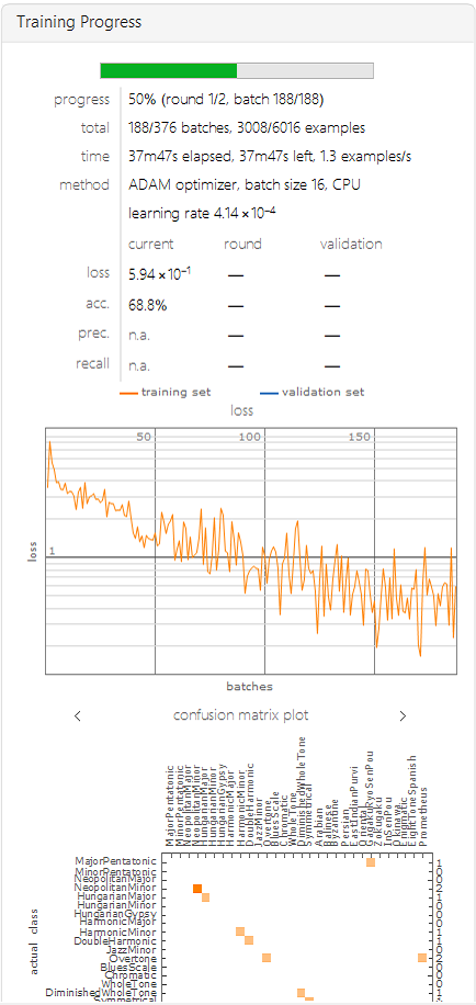
The network is ready to be trained. Below is an example of its learning:
trainedNet =
 NetTrain[newNet, samp, ValidationSet -> stest,
  TrainingProgressMeasurements -> {"ConfusionMatrixPlot", "Accuracy",
    "Precision", "Recall"},
  TrainingProgressCheckpointing -> {"Directory", dirModel},
  BatchSize -> 16, MaxTrainingRounds -> 2]
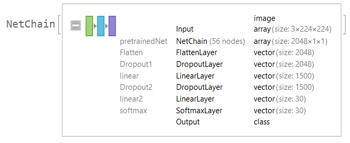
This was the final result of the learning:
We can save the resulting NetChain also in an .MX file with DumpSave so that we can use it when necessary:
filepath5 = FileNameJoin[{NotebookDirectory[], "trainedNet.mx"}];
DumpSave[filepath5, {trainedNet}];
With the code below we have, for example, the measures of global accuracy and the result of accuracy for each musical scale independently:
NetMeasurements[trainedNet, stest2 , "Accuracy"]
NetMeasurements[trainedNet, stest2, "F1Score"]
NetMeasurements[trainedNet, stest2, {<|"Measurement" -> "Precision",
   "ClassAveraging" -> "Macro"|>, <|"Measurement" -> "Recall",
   "ClassAveraging" -> "Macro"|>}]
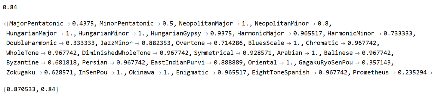
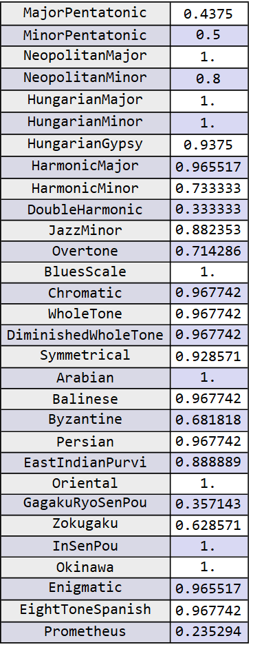
The same result of the independent scales measured separately, however, in the form of ResourceFunction[“NiceGrid”]:
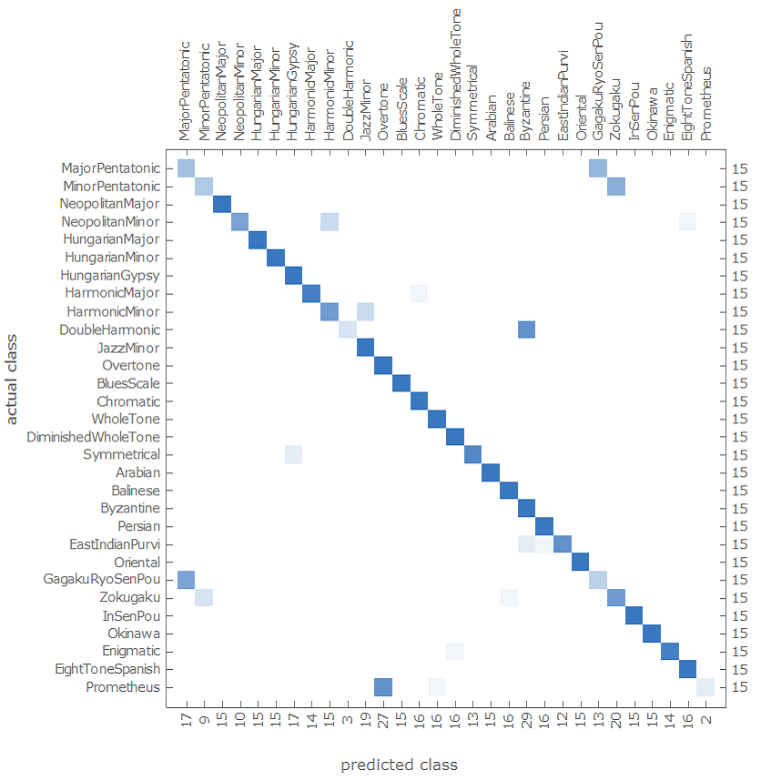
Let's see how the result of the ConfusionMatrixPlot of the customized ResNet was performing for the classes of musical scales:
NetMeasurements[trainedNet, stest2, "ConfusionMatrixPlot"]
To test the resulting custom NetChain, a function was created that generates a musical scale of choice and checks if the result was accurately predicted:
sampleMusic[scale_, opts_ : "Decision"] :=
 Module[{sound}, SetDirectory[NotebookDirectory[]];
  Get["trainedNet.mx"];
  scale -> {trainedNet[
      Rasterize[
       Spectrogram[
        sound = Sound@
          Table[ResourceFunction["MusicalScaleSample"][scale,
            "Tone" -> "C3", "NoteInterval" -> 0.17646,
            "Playing" -> "Mechanical"], 10], Frame -> None],
       RasterSize -> 600, ImageSize -> 300], opts] // Dataset, sound}]
For example:
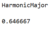
sampleMusic["JazzMinor"]
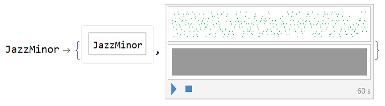
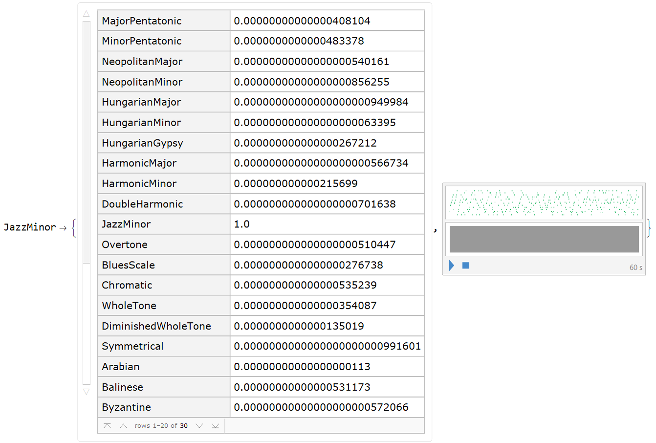
Above we see that it worked, the scale was recognized! Below is another sample of this class of musical scale with its probabilities:
sampleMusic["JazzMinor", "Probabilities"]
Conclusion (and Notes):
Although the methods have not been explored extensively (especially the first ones), we can have an idea of the results of each approach.
There are many other methods and options for each method, of course, in this work only a few were covered.
The best method by far was the customized ResNet, which was more carefully prepared and had very satisfactory results for most musical scales. Only 3 of the 30 scale classes had an accuracy below 50% and with the vast majority (23 of 30) above 70%.
It is clear that this work was a relatively simple work, in the sense that the conditions of recognition are controlled so that there is a satisfactory result, but nothing prevents the work from being extended to multiple situations in the future.
- Thanks: I would like to thank Siria Sadeddin, who gave me tips and guidance on the ResNet part. Thank you Siria!
Thank you!


