Introduction

Doing an internship with Wolfram Research Inc., we worked on the ASCII art project. We designed and developed four approaches to perform ASCII art. This post is about the first approach called an Intensity-based approach (the notebook is available as an attachment to the post).

When thinking about ASCII art generation, the first thing that comes to mind is to partition an image and see the partitions' similarity to the possible character set. In this case, the similarity measure is the mean intensity.

Approach

The approach uses the basic idea to partition an image into a rectangular grid and use intensities to assign a character raster to each cell (the result will always be a grayscale image).

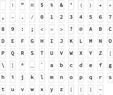
First of all, we need to rasterize all 95 ASCII characters (CharacterRange[" ", "~"]). We could do it as simple as Rasterize[#, options] /@ CharacterRange[" ", "~"], but this approach will require Rasterize to be called 95 times, which is pretty time-consuming. A workaround to accelerate the character rasters' generation is to call Rasterize once, via grouping all characters as a batch on a grid:

rasters = Rasterize[
    ExpressionCell[
        Grid[
            Partition[StandardForm[Framed[Style[#,
                            FontColor -> Black,
                            "FontSize" -> fontSize,
                            ScriptLevel -> 0,
                            TextAlignment -> Left,
                            Antialiasing -> True
                        ],
                        FrameStyle -> White,
                        FrameMargins -> 2
                    ]
                ] & /@ CharacterRange[" ", "~"],
                UpTo[12]
            ],
            ItemSize -> Full, Frame -> None
        ],
        {Background -> Transparent, "Inset", "Graphics", "Output"}
    ],
    "Image",
    System`ImageFormattingWidth -> Infinity,
    Background -> None
];

Now that we have all the characters rasters in one image, we can do a straight-forward image processing to separate them:

(* Split the grid into individual character boxes *)
rasters = Values @ ComponentMeasurements[{#, MorphologicalComponents @ FillingTransform[#]}, "Image"] & @ AlphaChannel[rasters];
		
(* Negate the character rasters, drop the margins, and crop as much as possible *)
rasters = ImageCrop[ImageTake[#, {3, -3}, {3, -3}], Padding -> White] & /@ ColorNegate[rasters];

(* Conform character rasters with respect to the largest character dimensions, ignoring whitespace *)
rasters = ImageCrop[#, Max /@ Transpose[ImageDimensions /@ Rest[rasters]], Padding -> White] & /@ rasters;

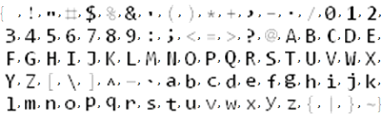
At this point, we have a list of all ASCII characters rasters, and we can sort them by their mean intensities to pick the "best match" concerning the position in the list rather than re-computing.

rasters = SortBy[rasters, ImageMeasurements[#, "MeanIntensity"]&];

We need to resize the input image if required (it is important to keep the ratio between the image and character raster dimensions to get something visually appealing), as well as to make sure it has a single grayscale channel:

image = RemoveAlphaChannel@ColorConvert[imageIn, "Grayscale"];
image = ImageResize[imageIn, resizeSize];

We can now partition the image; the partition dimensions is going to be the same as the resulting character raster one:

partitions = ImagePartition[image, ImageDimensions[First@rasters]];

To map each of the partitions to the corresponding character raster for the intensity similarity, we need to compute the partitions' intensities. Since we have already sorted the character rasters by their mean intensities, we can find the position of the closest value:

factor[i_] := Round[i * Length[rasters]];
intensityPositions = factor@ImageMeasurements[#, "MeanIntensity"] & /@ partitions;

intensityPositions at this point is already a nested list of indices of sorted character rasters list. We use intensityPositions to pick the corresponding character rasters and assemble the final ASCII art image:

ImageAssemble[Replace[intensityPositions, charIndex_ :> rasters[[Replace[charIndex, 0 -> 1]]], {2}]]    

Results

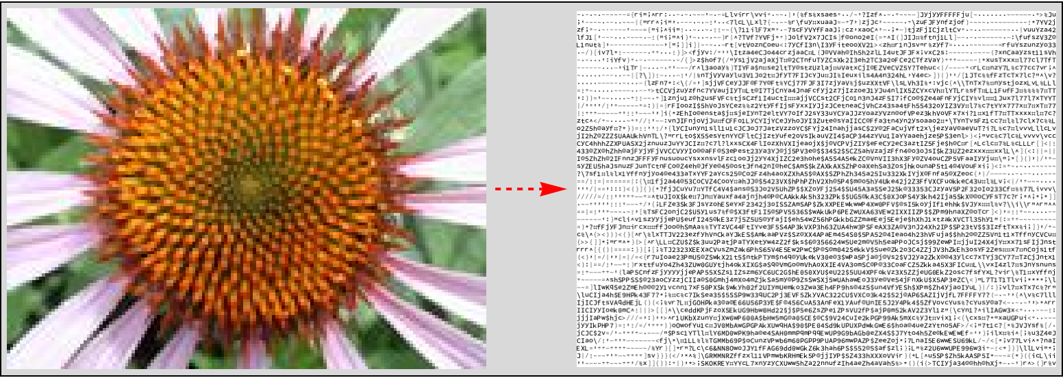
Below is a sample conversion for four images:

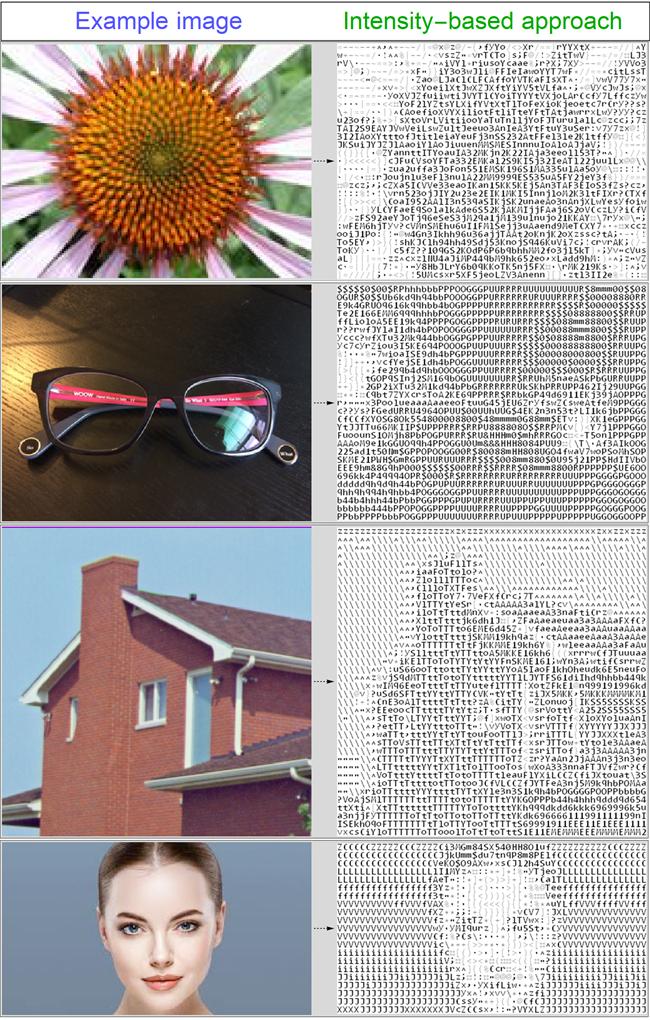
font size 15 resulted in character raster to have {10, 15} dimensions, resizing the input image to match 500 in one dimension

Another Wolfram community post that proposed a framework to perform ASCII art. Let us see how we compare (visually):

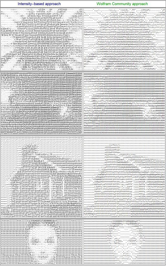
font size 15 resulted in character raster to have {10, 15} dimensions, resizing the input image to match 500 in one dimension

As we can see, the results are similar, but in the Intensity-based approach, edges are more precise.

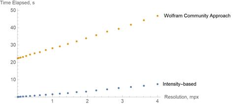
For time-complexity Comparison, a square image, which resolution was changing from 100 to 2000. Approaches used the same values for similar parameters (the time computation uses AbsoluteTiming). Also, we modified the procedures to import already rasterized characters, so only algorithm complexity is considered:

Conclusion

As we can see, the Intensity-based approach is way faster.

Overall this approach cannot recover the partition structure and the character raster (since it only uses the mean intensity value as a distance measure).

References & Credits

• ASCII art: Wikipedia
• ASCII?: Convert Images and GIFs into ASCII Art.
• Convolution-based approach ASCII art
• Classifier-based approach ASCII art
• Image mosaic using convolution

Thanks to Wolfram Team and Mikayel Egibyan in particular for mentoring the internship.

Attachments:

ImageToAscii.nb