Dear Community,

I would like to ask your help again. Related to the problem above, I would like to define the PDF and CDF of the following events:

X1 and X2 are random variable from normal distributions with equal sigma and mu1 <= mu2.

What is the conditional distribution of X1 when X1>X2?

As I have programming background, I've made a simulation in R:

mu1 <- 0
mu2 <- 3
r.u1 <- rnorm(n = 10000000, mean = mu1, sd = sigma)
r.u2 <- rnorm(n = 10000000, mean = mu2, sd = sigma)
RS2.u1 <- dnorm(xx, mean = mu1, sd = s1)
RS3.u2 <- dnorm(xx, mean = mu2, sd = s2)
tt <- as.data.frame(cbind(r.u1, r.u2, collision = r.u1 > r.u2))
hh <- hist(tt[tt$collision == 1,"r.u2"], freq = F, breaks = xx, xlim = c(-10, 10))

    ![enter image description here][1]

To figure out the CDF first in Mathematica, my attempt was:

distX = (1/Sqrt[2 Pi \[Sigma]1^2]) Exp[-((x - \[Mu]1)/\[Sigma]1)^2/2]
distY = (1/Sqrt[2 Pi \[Sigma]1^2]) Exp[-((y - \[Mu]1)/\[Sigma]1)^2/2]

distXminusY = 
 Assuming[\[Sigma] > 0, 
  TransformedDistribution[
   x - y, {x \[Distributed] NormalDistribution[\[Mu]1, \[Sigma]], 
    y \[Distributed] NormalDistribution[\[Mu]2, \[Sigma]]}]]

dist_condyx = 
 Assuming[Element[{\[Mu]1, \[Mu]2, \[Sigma]1}, Reals] && \[Sigma]1 > 
    0 , Integrate[
   distX[t]*(1 - CDF[distY, t])/CDF[distXminusY, 0], {t, -Infinity, 
    x}]]

It seems it can't integrate the function but maybe I define it incorrectly. To get the PDF I have to derivate this function afterwards.

Can you advise me how to proceed with this?

Many thanks for your help.

Best, Attila

Attachments:

Screen Shot 2021...png

The direct approach would be to try to determine the cdf of x1 conditional on x1 > x2:

cdf = Probability[x1 <= x0 \[Conditioned] x1 > x2,
  {x1 \[Distributed] NormalDistribution[mu1, sigma1],
   x2 \[Distributed] NormalDistribution[mu2, sigma2]},
  Assumptions -> {mu1 <= mu2, sigma1 > 0, sigma2 > 0}]

But this just returns the command. This is either because Probability doesn't know how to obtain the answer or because there is no closed-form answer. So more basic approaches are needed.

We first determine the joint pdf of x1 and x2 given that x1 > x2 and then integrate over x2 to get the pdf of x1 conditional on x1 > x2.

(* Probability that x1 > x2 *)
p = Probability[x1 > x2,
  {x1 \[Distributed] NormalDistribution[mu1, sigma1],
   x2 \[Distributed] NormalDistribution[mu2, sigma2]},
  Assumptions -> {sigma1 > 0, sigma2 > 0}]
(* 1/2 Erfc[(mu1 - mu2)/(Sqrt[2] Sqrt[sigma1^2 + sigma2^2])] *)

(* Joint distribution of x1 and x2 given that x1 > x2 *)
jointPDF = Piecewise[{{PDF[NormalDistribution[mu1, sigma1], x1]*
     PDF[NormalDistribution[mu2, sigma2], x2]/p, x1 > x2}}, 0]

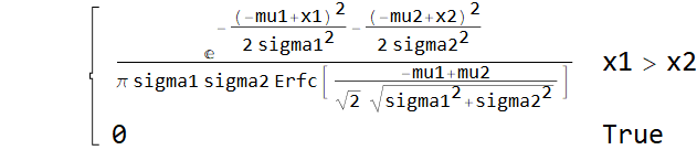
(* Integrate over x2 to get marginal pdf for x1 given that x1 > x2 *)
pdfx1 = Integrate[jointPDF, {x2, -Infinity, x1},
  Assumptions -> {x1 \[Element] Reals, mu1 <= mu2, sigma1 > 0, 
    sigma2 > 0}]
(* (E^(-((mu1 - x1)^2/(2 sigma1^2)))*
  Erfc[(mu2 - x1)/(Sqrt[2] sigma2)])/(Sqrt[2 \[Pi]] sigma1 Erfc[(-mu1 + mu2)/(Sqrt[2] Sqrt[sigma1^2 + sigma2^2])]) *)

There doesn't appear to be a nice closed form for the cdf, mean, or variance.

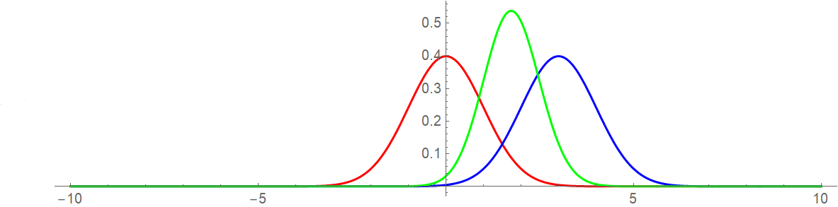
This does appear to match what you got from R:

parms = {mu1 -> 0, mu2 -> 3, sigma1 -> 1, sigma2 -> 1};
Plot[{PDF[NormalDistribution[mu1, sigma1] /. parms, x1],
  PDF[NormalDistribution[mu2, sigma2] /. parms, x1],
  pdfx1 /. parms}, {x1, -10, 10},
 PlotStyle -> {Red, Blue, Green}, PlotRange -> All, AspectRatio -> 1/4]

Yes, that is how to get the marginal distribution of x2 given that x1 > x2.

But I would avoid the statement "X2 distribution restricts everything" because one could just as easily (and incorrectly) state that the "X1 distribution restricts everything" as one could rephrase your other statement as "x2 can't go further as it bumps into x1." I would say that such a "cause-and-effect" statement is both wrong and unnecessary.

PDF[distCensored, z]

just returns the code (i.e., Mathematica can't figure it out). But because distXminusY is just a normal distribution the pdf of distCensored is found with defining a piecewise function:

pdf[z_] := Piecewise[{{PDF[distXminusY, z]/CDF[distXminusY, 0], z <= 0}}, 0]

Many thanks for your advice. My purpose is to define the PDF of the difference of two gaussian random variables (X and Y) if X-Y<0 and see the mean and variance. At this stage I just really want to learn how to define a custom PDF and ask for the mean and variance.

pdfx[x_] = 
 ConditionalExpression[
  PDF[(1/Sqrt[2*Pi]*\[Sigma]1) *(E^-1/
       2*((x - \[Mu]1)/\[Sigma]1)^2), {x, -Infinity, 
    Infinity}], \[Sigma]1 > 0]

Mean[pdfx]

and

Variance[pdfx]

It would be helpful if you posted actual code rather than a picture. And should the y be an x?

Also, if you describe a bit more what you want to do (in words), then more of us could probably give you something explicit.

I wonder if you mean to write the following:

dist = ProbabilityDistribution[(1/Sqrt[2 Pi \[Sigma]1^2]) Exp[-((x - \[Mu]1)/\[Sigma]1)^2/2],
   {x, -Infinity, Infinity}, Assumptions -> \[Sigma]1 > 0];
PDF[dist, x]
(* E^(-((x - \[Mu]1)^2/(2 \[Sigma]1^2)))/(Sqrt[2 \[Pi]] Sqrt[\[Sigma]1^2] *)
Mean[dist]
(* \[Mu]1 *)
Variance[dist]
(* \[Sigma]1^2 *)