OMG! Of course my mini-example has nothing to do with your problem. You asked how to mark and label points in some plot, and I told you.

Hence you did not ask for marking points, but for finding them, i.e. solving your problem. See my post dated 01.03.2021, "Point 4: Your actual problem". There I gave you complete answer and coding.

BTW: Meanwhile I read your original paper and found that:

1. Your function definition seems to be wrong.
2. Your problem posing is definetly wrong.

I have resumed work on your problem and collected everything in a notebook. I will soon come up with a post that includes this notebook. It will solve your problem completely and correctly.

Very interesting post and notebook DiracKasten1.nb. Of course you are right concerning the problem posing. We search for solutions of the complex equations of T11 == 0, not Re[T11] == 0 as Affaa told us originally.

I did not check whether T11 should be T22. I believe you are right. But its just naming in our context.

Really? Ok. What is wrong in my notebook DiracKasten1.nb? But as Werner said, that is not really important. The task is to find Re[ T11 ] = 0 (T11 being actually T22 - or not?) and simultaneously Im[ T11 ] = 0, and I don't see that this problem is solved.

However, the results have been shown in the journal

But they don't say how they got their results. With the help of Mathematica. Wow. They should have described what they did (or publish a code).

I think you should contact the author(s) and ask them (and direct their attention to this thread).

Seriously ??

I will study problem solving which you will show you later.

I am very grateful in advance, Werner Geiger.

I have got this picture, how do I mark the point of intersection between the blue and black lines as the green mark / point on the chart shown by Werner Geiger?

I'm sorry for my limited knowledge of programming / coding so I keep asking questions.

How do I get an expression with the integer value n in the solution or plot? Will it be the same or close to the plot in the source of my journal?

@Affaa Nam, posting a question with unclear details and/or purpose can make others confused and will result in unwanted responses. Please take time to think through the answers and suggestions offered by other members here. If you are still in need of an assistance, then make sure you pinpoint your problem and state it as clearly as possible so that others will have a decent chance to assist.

Yes Hans is correct. You do not have an equation. You have an expression (which is only one side of an equation). You are defining a variable f[En,Va] with that expression. You need to show the original problem from the textbook or source that you have because you are missing elements in your questions that will allow us to give you a complete solution. The problem itself does not seem overly difficult, but there does seem to be missing information.

I have said that

I consider the definition of T to be a function of f[En_], because the value I want to find is the value of En

The initial condition is

f [ En, Va ] = Re [ f [ En, Va ] ] + Im [ f [ En, Va ] ] = 0

As it turned out, after the plot was formed, only the plot of the "Real" section was similar to the plot in my reading source. So, I think the condition changed to

Re [ f [ En, Va ] ] = 0.

n in my table means the energy level, because the En variable I meant from the start is actually the eigen / energy value. However, I also do not understand how to generate it from a Wolfram Mathematica encoding result. I had thought that maybe the results obtained from the Wolfram Mathematica coding were only in the form of a plot, while the table was created manually by entering the specified coordinate values.

Maybe I need to tell you that I encountered this problem when I read an article / journal, then I tried to study it and found the incomprehension that I asked about. What if I tell / send the journal / article that I am studying so you can understand what I mean and my problem becomes clear? :(

Thanks for your explanation. But I still do not understand what you want to do. Given your function

f [ En, Va ]

do you want those En and Va where

Re [ f [ En, Va ] ] == 0

as Werner pointed out or

Re [ f [ En, Va ] ] == Im [ f [ En, Va ] ]

Point 1: My mistake

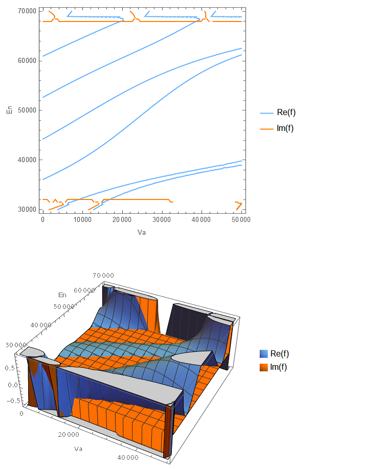
First of all remove the Evaluate within my definition of f. This is not correct. It does not change the function values but the contour-plot. The plots now look like (To get the same colors for real and imaginary parts in both plots I added explicit colors cols={RGBColor[0.4, 0.7, 1], RGBColor[1, 0.5, 0]} for ContourStyle and PlotStyle):

Point 2: Strange table-values

I don't understand why your table does not show values like mine. Maybe executing a Clear["Global'*"] might help.

BTW: It is never a good idea to use symbols starting with uppercase letters. Your Va and En shoul better read va and en.

Point 3: Global function definition

For not repeating the definition of function f again and again, I define it as global now. (This could be simplified for avoiding the same calculations over and over again). You must execute this one times:

Clear[f];
f[Va_, En_] := 
  Module[{Vb = 50000, a = 0.01, b = 0.02, c = 137.036, k, p, q, A, B, 
    H},
   k = Sqrt[En^2 - c^4]/c; 
   p = Sqrt[(En + c^2 - Va)*(En - c^2 - Va)]/c; 
   q = Sqrt[(En + c^2 - Vb)*(En - c^2 - Vb)]/c; 
   A = Sqrt[(En - c^2)/(En + c^2)]; 
   B = Sqrt[(En - c^2 - Vb)/(En + c^2 - Vb)]; 
   H = Sqrt[(En - c^2 - Va)/(En + c^2 - Va)];
   Simplify[
    (E^(I*q*b)/(16*A^2*B*H)*
      (((A + H)^2)*((A + B)^2*E^(2*I*(k*(a - b) - p*a)) - (A - B)^2*
            E^(-2*I*(k*(a - b) - p*a))) + ((A - H)^2)*((A - B)^2*
            E^(-2*I*(k*(a - b) + p*a)) - (A + B)^2*
            E^(2*I*(k*(a - b) + p*a))) + 
        2*(A^2 - B^2)*(A^2 - H^2)*(E^(2*I*p*a) - E^(-2*I*p*a))))]
   ];

Our program now looks like:

If[True, Block[{En, Va, tab, 
    cols = {RGBColor[0.4, 0.7, 1], RGBColor[1, 0.5, 0]}},
   (* Define function; f is defined globally *)
   If[False, Print[f[Va, En]]];

   (* Print a table with function-values *)
   tab = Table[Column[Round[ReIm[f[Va, En]], 0.01], Center]
     , {Va, 0, 50000, 5000}, {En, 30000, 70000, 4000}];
   Print[Grid[Join[
      {Prepend[Range[30000, 70000, 4000], "Va\\En:"]},
      Join[Transpose[{Range[0, 50000, 5000]}], tab, 2]],
     Dividers -> {{2 -> True}, {1 -> True, 2 -> True}}]];

   (* Show real and imaginary part of function-values *)
   Print[ContourPlot[{Re[f[Va, En]], Im[f[Va, En]]}, {Va, 0, 
      50000}, {En, 30000, 70000},
     PlotRange -> All,
     ContourStyle -> cols,
     PlotPoints -> {50, 40}, MaxRecursion -> 2,
     FrameLabel -> {"Va", "En"}, PlotLegends -> {"Re(f)", "Im(f)"}
     ]];
   (* Show real and imaginary part of function-values in 3D *)
   Print[Plot3D[{Re[f[Va, En]], Im[f[Va, En]]}, {Va, 0, 50000}, {En, 
      30000, 70000},
     PlotRange -> {All, All, Automatic},
     PlotStyle -> cols,
     PlotPoints -> {50, 40}, MaxRecursion -> 2,
     AxesLabel -> {"Va", "En"}, PlotLegends -> {"Re(f)", "Im(f)"}
     ]];
   ]];

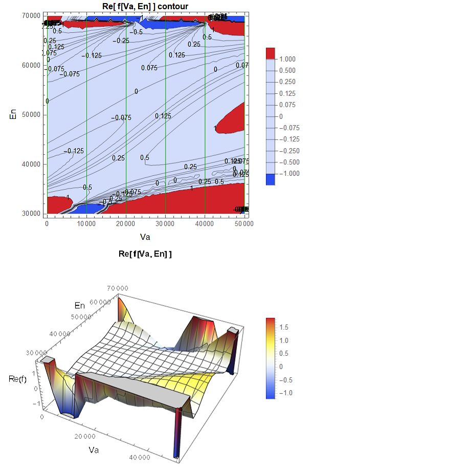
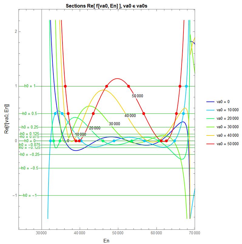
Point 4: Your actual problem

If I understand you correctly, you are looking for the solution of Re[ f[va0, En] ] == h0 for any given value of va0 and h0.

First of all we redraw the contour- and 3D plots of the real part and add some more information on it including the desired va0 and h0 values.

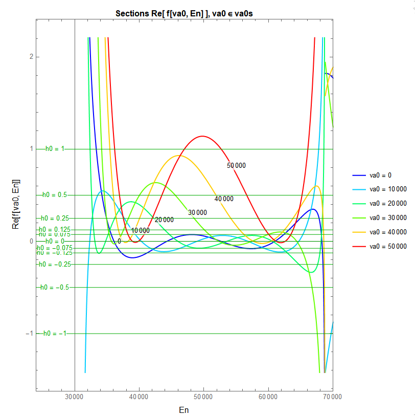
In addition we draw another plot with the sections Re[ f[va0, En] ] of our function for the desired va0 values.

If[True, Block[{En, Va, va0s, cntVa0s, h0s, cntH0s, prVa = {0, 50000},
     prEn = {30000, 70000}, prEnL = 6000, col},
   (* Desired Va values and function heights *)
   va0s = Range[First[prVa], Last[prVa], 10000]; 
   cntVa0s = Length[va0s];
   h0s = {-1, -0.5, -0.25, -0.125, -0.075, 0, 0.075, 0.125, 0.25, 0.5,
      1}; cntH0s = Length[h0s];
   (* Show real part Re(f) of function values *)
   Print[ContourPlot[Re[f[Va, En]]
     , {Va, First[prVa], Last[prVa]}, {En, First[prEn], Last[prEn]},
     PlotRange -> All,
     Contours -> h0s, ContourLabels -> True,
     ColorFunction -> "TemperatureMap",
     PerformanceGoal -> "Quality",
     FrameLabel -> (Style[#, Black, Larger] & /@ {"Va", "En"}),
     PlotLegends -> Automatic,
     PlotLabel -> Style["Re[ f[Va, En] ] contour", Black, Bold],
     Epilog -> {Darker[Green], Thin, 
       Line[{{#, First[prEn]}, {#, Last[prEn]}} & /@ va0s]}
     ]];
   (* Show real part Re(f) of function values in 3D *)
   Print[Plot3D[Re[f[Va, En]]
     , {Va, First[prVa], Last[prVa]}, {En, First[prEn], Last[prEn]},
     PlotRange -> {All, All, Automatic},
     ColorFunction -> "TemperatureMap",
     PerformanceGoal -> "Quality",
     AxesLabel -> (Style[#, Black, Larger] & /@ {"Va", "En", "Re(f)"}),
     PlotLegends -> Automatic,
     PlotLabel -> Style["Re[ f[Va, En] ]", Black, Bold]
     ]];
   (* Show sections through Re(f) at the points va0 *)
   col[va_] := 
    Hue[2/3 + (0 - 2/3)/(Last[prVa] - First[prVa])*(va - First[prVa])];
   Print[Plot[Evaluate[Table[Re[f[va0, En]], {va0, va0s}]]
     , {En, First[prEn], Last[prEn]},
     PlotRange -> {prEn - {prEnL, 0}, Automatic}, 
     AxesOrigin -> {First[prEn], 0},
     PerformanceGoal -> "Quality",
     PlotStyle -> (col[#] & /@ va0s),
     Frame -> True, 
     FrameLabel -> (Style[#, Black, Larger] & /@ {"En", 
         "Re[f[va0, En]]"}),
     PlotLegends -> (Style[Row[{"va0 = ", #}], 10] & /@ va0s), 
     PlotLabels -> 
      Placed[va0s, {Scaled[#/10], Above} & /@ Range[cntVa0s]],
     PlotLabel -> 
      Style["Sections Re[ f[va0, En] ], va0 \[Element] va0s", Black, 
       Bold],
     ImageSize -> Scaled[0.85], AspectRatio -> 5/4,
     Epilog -> {Darker[Green], Thin,
       Line[{{First[prEn] - prEnL, #}, {Last[prEn], #}} & /@ h0s],
       Inset[
          Style[Row[{"h0 = ", #}], 10, ![enter image description here][2]
           Background -> White], {First[prEn] - prEnL/2, #}, {0, 
           0}] & /@ h0s}
     ]];
   ]];

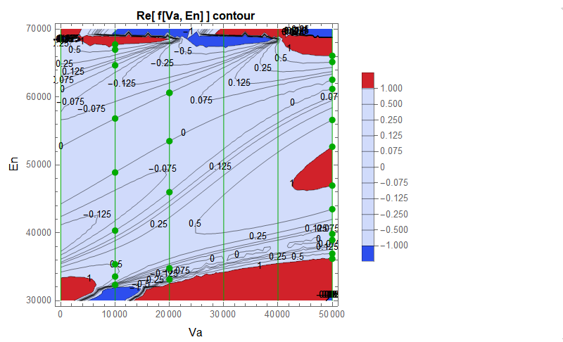
Then we solve the equations Re[ f[va0, En] ] == h0 for some given values va0 an h0. We define a new global function r[Va_ ,En_ ] for the simplified real part Re[ f[va0, En] ].

Solve is not able to solve that, hence we use NSolve. But this does not terminate within reasonable time (Interrupt wit Alt+.).

So we try to find solutions with FindRoot, which takes an approximation per solution. We roughly lookup the approximations in the previous section-plot. They are given as an association solApproxs = <| {va0,h0} -> {En01, En02, ...}, ... |>. For each {va0,h0}-pair there is a list with zero to n En-approximations. Note: I defined only some solution approximations, not all of them.

In the same way, we collect the solutions within an association sols = <| {va0,h0} -> {En1, En2, ...}, ... |> for later use. For each {va0,h0}-pair there is a list with zero to n En-solutions.

Finally we draw our contour- and section plot again exactly like before, but with the solutions marked by points.

Clear[r];
r[Va_, En_] := Simplify[Re[f[Va, En]]];

If[True, Block[{test = False, En, Va, va0s, cntVa0s, h0s, cntH0s, 
    prVa = {0, 50000}, prEn = {30000, 70000}, prEnL = 6000, 
    solApproxs, approxs, sols, sol, col, va0},
   (* Desired Va values and function heights *)
   va0s = Range[First[prVa], Last[prVa], 10000]; 
   cntVa0s = Length[va0s];
   h0s = {-1, -0.5, -0.25, -0.125, -0.075, 0, 0.075, 0.125, 0.25, 0.5,
      1}; cntH0s = Length[h0s];

   (* From the plots take some approximations of the solutions for \
{va0,h0} *)
   solApproxs = <|{50000, 1} -> {36000, 44000, 59000, 65000}, {50000, 
       0.5} -> {37000, 43000, 59000, 65000}, {50000, 0} -> {38000, 
       41000, 61000, 63000},
     {20000, 0} -> {34000, 37000, 46000, 53000, 62000, 65000},
     {10000, 1} -> {68000}, {10000, 0.5} -> {33000, 36000, 
       67000}, {10000, 0} -> {33000, 40000, 49000, 59000, 66000}|>;

   (* Solve the equations Re[f[va0,En]] \[Equal] 
   h0 for given values va0 and h0. *)
   (* Collect the solutions within sols *)
   sols = 
    Association[
     Flatten[Table[{va0, h0} -> {}, {va0, va0s}, {h0, h0s}]]];
   Do[(* va0 *)
    If[test && ! MemberQ[{50000, 20000, 10000}, va0], Continue[]];
    Do[(* h0 *)
     If[test && ! MemberQ[{1, 0.5, 0(*,-0.075*)}, h0], Continue[]];
     Print[
      Style[Row[{"Solving for va0 = ", va0, ", h0 = ", h0}], Blue, 
       Bold]];
     (* sol=Solve[r[va0,En]\[Equal]h0,En]; does not work *)
     (*sol=NSolve[r[va0,En]\[Equal]h0&&En\[Element]Reals&&First[
     prEn]\[LessEqual]En\[LessEqual]Last[prEn],En,Complexes]; 
     does not terminate *)
     approxs = solApproxs[{va0, h0}];
     If[MissingQ[approxs],
      Print["No approximation known!"]
      ,
      Do[(* approx *)
        sol = FindRoot[r[va0, En] == h0, {En, approx}];
        If[test, Echo[{approx, sol}, "{approx,sol}: "]];
        AppendTo[sols[{va0, h0}], En /. First[sol]]
        , {approx, approxs}];
      ];
     (* just for beauty *)
     sols[{va0, h0}] = Sort[DeleteDuplicates[sols[{va0, h0}]]];
     Print[Row[{"Solutions En = ", sols[{va0, h0}]}]]
     , {h0, h0s}]
    , {va0, va0s}];
   If[test && False, 
    Print["All solutions En =\n", Column[Normal[sols]]]];

   (* Show real part Re(f) of function values with solutions marked *)


   Print[ContourPlot[r[Va, En]
     , {Va, First[prVa], Last[prVa]}, {En, First[prEn], Last[prEn]},
     PlotRange -> All,
     Contours -> h0s, ContourLabels -> True,
     ColorFunction -> "TemperatureMap",
     PerformanceGoal -> "Quality",
     FrameLabel -> (Style[#, Black, Larger] & /@ {"Va", "En"}),
     PlotLegends -> Automatic,
     PlotLabel -> Style["Re[ f[Va, En] ] contour", Black, Bold],
     Epilog -> {Darker[Green], Thin, 
       Line[{{#, First[prEn]}, {#, Last[prEn]}} & /@ va0s],
       PointSize[Large], 
       Point[Flatten[
         Table[If[
           sols[{va0, h0}] != {}, {va0, #} & /@ sols[{va0, h0}], 
           Nothing], {va0, va0s}, {h0, h0s}], 2]]}
     ]];
   (* Show sections through Re(f) at the points va0 with solutions \
marked *)
   col[va_] := 
    Hue[2/3 + (0 - 2/3)/(Last[prVa] - First[prVa])*(va - First[prVa])];
   Print[Plot[Evaluate[Table[r[va0, En], {va0, va0s}]]
     , {En, First[prEn], Last[prEn]},
     PlotRange -> {prEn - {prEnL, 0}, Automatic}, 
     AxesOrigin -> {First[prEn], 0},
     PerformanceGoal -> "Quality",
     PlotStyle -> (col[#] & /@ va0s),
     Frame -> True, 
     FrameLabel -> (Style[#, Black, Larger] & /@ {"En", 
         "Re[f[va0, En]]"}),
     PlotLegends -> (Style[Row[{"va0 = ", #}], 10] & /@ va0s), 
     PlotLabels -> 
      Placed[va0s, {Scaled[#/10], Above} & /@ Range[cntVa0s]],
     PlotLabel -> 
      Style["Sections Re[ f[va0, En] ], va0 \[Element] va0s", Black, 
       Bold],
     ImageSize -> Scaled[0.85], AspectRatio -> 5/4,
     Epilog -> {Darker[Green], Thin,
       Line[{{First[prEn] - prEnL, #}, {Last[prEn], #}} & /@ h0s],
       Inset[
          Style[Row[{"h0 = ", #}], 10, 
           Background -> White], {First[prEn] - prEnL/2, #}, {0, 
           0}] & /@ h0s,
       PointSize[Large],
       {va0 = #; col[va0],

          Point[Flatten[
            Table[If[
              sols[{va0, h0}] != {}, {#, h0} & /@ sols[{va0, h0}], 
              Nothing], {h0, h0s}], 1]]} & /@ va0s }
     ]];
   ]];

I think, your problem is solved by this approach. At least numerically. I don't know if there is a closed analytical solution. Probably one would have to simplify the function significantly manually. With Simplify it is still too complicated.

As Werner pointed out your f[En_] is somewhat strange.

Type for example (after your code has run) f[50000]. What do you get?

What about telling us what exactly your problem is. Perhaps there is an alternative way to find a solution?

By the way: The function becomes more vivid if you plot it in 3D:

(* Show real and imaginary part of function-values in 3D *)
Print[Plot3D[{Re[f[Va, En]], Im[f[Va, En]]}, {Va, 0, 50000}, {En, 
    30000, 70000},
   PlotRange -> {All, All, Automatic},
   PlotPoints -> {50, 40}, MaxRecursion -> 2,
   AxesLabel -> {"Va", "En"}, PlotLegends -> {"Re(f)", Im["f"]}]];

No, you did not define them. There they are variables to be used by ContourPlot, and as far as I know they are local to the plot-routine. So in your Point statement both have no value. Look at your error message, there appears En , without a value of course.

Try your ContourPlot without Point[{Va, En}] and there will be no error.

Go with the pointer unto your plot, then do a right mouse-click, a window opens. click Get Cooridinates and you can chose any region of the plot with your mouse.

Do as said above (GetCoordinates), move to the point of interest, then left mouse-click, then Ctrl-C, then same procedure at the next point and so on. Finally move to an empty cell and use Ctrl-V. A list of the points chosen will appear. You can of course give it a name: type for example pts = Ctrl-V

What do you mean by

Point[{Va, En}]

Here Va and En are not defined!