I have written extensively about statistical arbitrage strategies in other posts, for example:
In this postI want to focus on applications of machine learning in stat arb and pairs trading, including genetic algorithms, deep neural networks and reinforcement learning.
Pair Selection
Let's begin with the subject of pairs selection, to set the scene. The way this is typically handled is by looking at historical correlations and cointegration in a large universe of pairs. But there are serious issues with this approach, as described in this post:
Instead I use a metric that I call the correlation signal, which I find to be a more reliable indicator of co-movement in the underlying asset processes. I wont delve into the details here, but you can get the gist from the following: 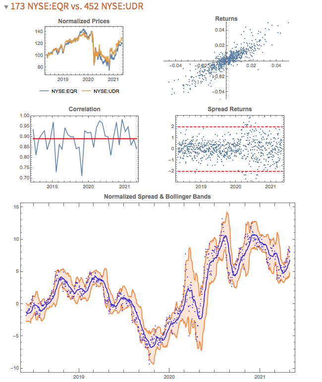 The search algorithm considers pairs in the S&P 500 membership and ranks them in descending order of correlation information. Pairs with the highest values (typically of the order of 100, or greater) tend to be variants of the same underlying stock, such as GOOG vs GOOGL, which is an indication that the metric "works" (albeit that such pairs offer few opportunities at low frequency). The pair we are considering here has a correlation signal value of around 14, which is also very high indeed. Trading Strategy Development
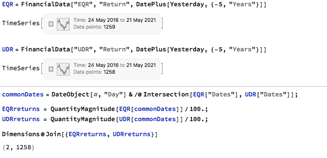
We begin by collecting five years of returns series for the two stocks:
The first approach we'll consider is the unadjusted spread, being the difference in returns between the two series, from which we crate a normalized spread "price", as follows.
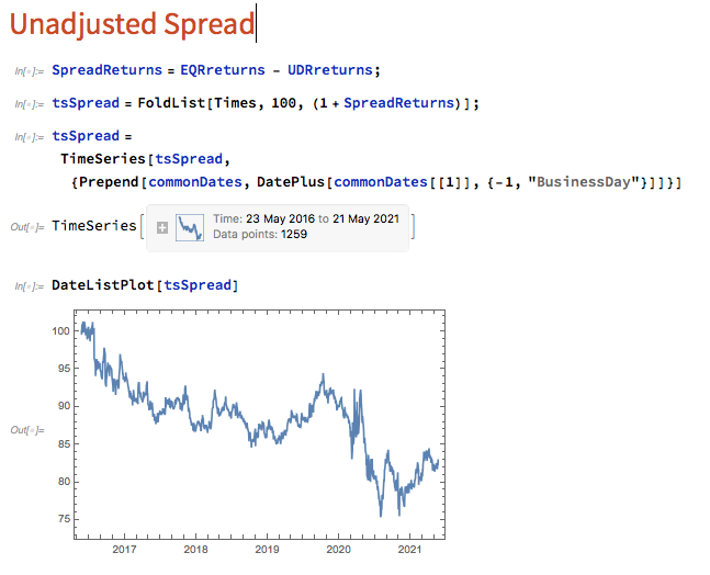
This methodology is frowned upon as the resultant spread is unlikely to be stationary, as you can see for this example in the above chart. But it does have one major advantage in terms of implementation: the same dollar value is invested in both long and short legs of the spread, making it the most efficient approach in terms of margin utilization and capital cost - other approaches entail incurring an imbalance in the dollar value of the two legs.
But back to nonstationarity. The problem is that our spread price series looks like any other asset price process - it trends over long periods and tends to wander arbitrarily far from its starting point. This is NOT the outcome that most statistical arbitrageurs are looking to achieve. On the contrary, what they want to see is a stationary process that will tend to revert to its mean value whenever it moves too far in one direction.
Still, this doesn't necessarily determine that this approach is without merit. Indeed, it is a very typical trading strategy amongst futures traders for example, who are often looking for just such behavior in their trend-following strategies. Their argument would be that futures spreads (which are often constructed like this) exhibit clearer, longer lasting and more durable trends than in the underlying futures contracts, with lower volatility and market risk, due to the offsetting positions in the two legs. The argument has merit, no doubt. That said, spreads of this kind can nonetheless be extremely volatile.
So how do we trade such a spread? One idea is to add machine learning into the mix and build trading systems that will seek to capitalize on long term trends. We can do that in several ways, one of which is to apply genetic programming techniques to generate potential strategies that we can backtest and evaluate. For more detail on the methodology, see:
I built an entire hedge fund using this approach in the early 2000's (when machine learning was entirely unknown to the general investing public). These days there are some excellent software applications for generating trading systems and I particularly like Mike Bryant's Adaptrade Builder, which was used to create the strategies shown below:
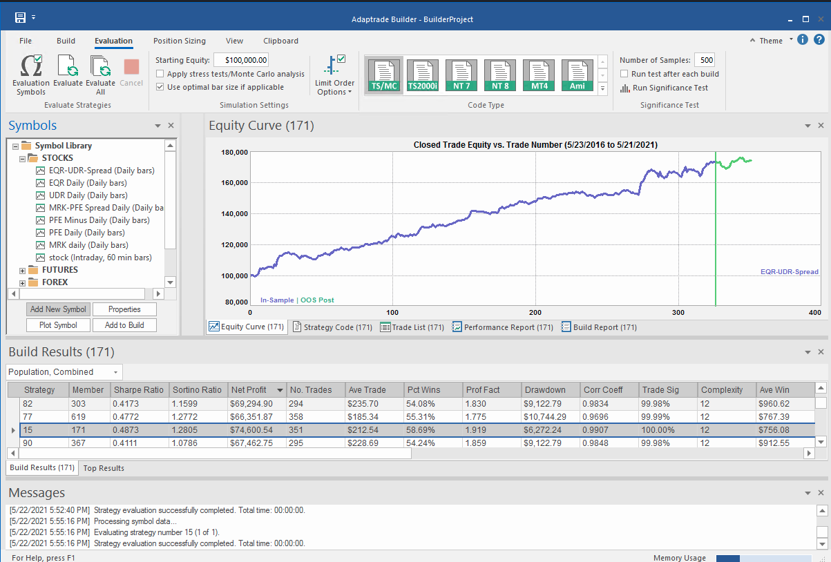
Builder has no difficulty finding strategies that produce a smooth equity curve, with decent returns, low drawdowns and acceptable Sharpe Ratios and Profit Factors - at least in backtest! Of course, there is a way to go here in terms of evaluating such strategies and proving their robustness. But it's an excellent starting point for further R&D.
But let's move on to consider the "standard model" for pairs trading. The way this works is that we consider a linear model of the form
**Y(t) = beta * X(t) + e(t)**
Where Y(t) is the returns series for stock 1, X(t) is the returns series in stock 2, e(t) is a stationary random error process and beta (is this model) is a constant that expresses the linear relationship between the two asset processes. The idea is that we can form a spread process that is stationary:
**Y(t) - beta * X(t) = e(t)**
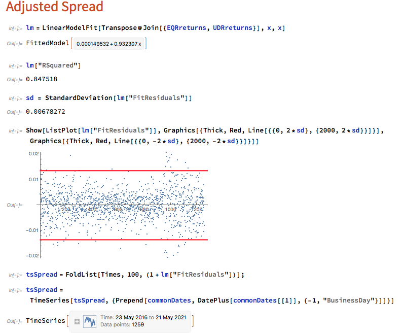
In this case we estimate beta by linear regression to be 0.93. The residual spread process has a mean very close to zero, and the spread price process remains within a range, which means that we can buy it when it gets too low, or sell it when it becomes too high, in the expectation that it will revert to the mean:
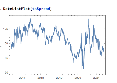
In this approach, "buying the spread" means purchasing shares to the value of, say, USD 1 million in stock 1, and selling beta * USD 1 Million of stock 2 (around $930,000). While there is a net dollar imbalance in the dollar value of the two legs, the margin impact tends to be very small indeed, while the overall portfolio is much more stable, as we have seen.
The classical procedure is to buy the spread when the spread return falls 2 standard deviations below zero, and sell the spread when it exceeds 2 standard deviations to the upside. But that leaves a lot of unanswered questions, such as:
- After you buy the spread, when should you sell it?
- Should you use a profit target?
- Where should you set a stop-loss?
- Do you increase your position when you get repeated signals to go
long (or short)?
- Should you use a single, or multiple entry/exit levels?
And so on - there are a lot of strategy components to consider. Once again, we'll let genetic programming do the heavy lifting for us:
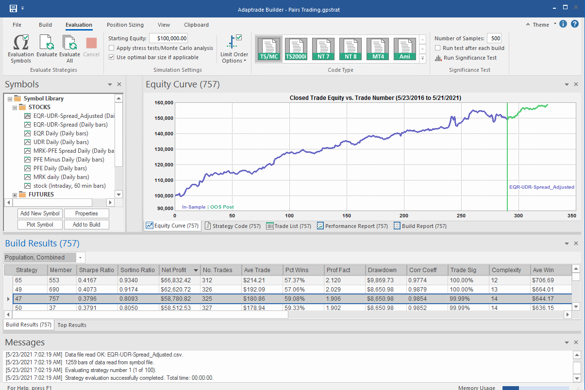
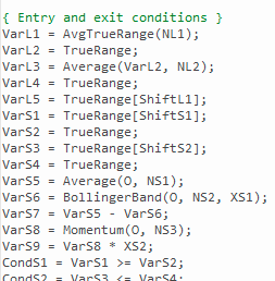
What's interesting here is that the strategy selected by the Builder application makes use of the Bollinger Band indicator, one of the most common tools used for trading spreads, especially when stationary (although note that it prefers to use the Opening price, rather than the usual close price):
Ok so far, but in fact I cheated! I used the entire data series to estimate the beta coefficient, which is effectively feeding forward-information into our model. In reality, the data comes at us one day at a time and we are required to re-estimate the beta every day.
Let's approximate the real-life situation by re-estimating beta, one day at a time. I am using an expanding window to do this (i.e. using the entire data series up to each day t), but is also common to use a fixed window size to give a "rolling" estimate of beta in which the latest data plays a more prominent part in the estimation. The process now looks like this:
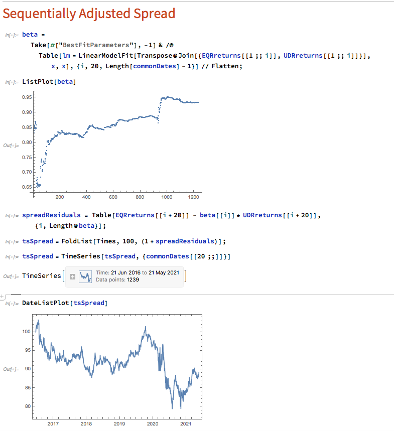
Here we use OLS to produce a revised estimate of beta on each trading day. So our model now becomes:
**Y(t) = beta(t) * X(t) + e(t)**
i.e. beta is now time-varying, as can be seen from the chart above.
The synthetic spread price appears to be stationary (we can test this), although perhaps not to the same degree as in the previous example, where we used the entire data series to estimate a single, constant beta. So we might anticipate that out ML algorithm would experience greater difficulty producing attractive trading models. But, not a bit of it - it turns out that we are able to produce systems that are just as high performing as before:
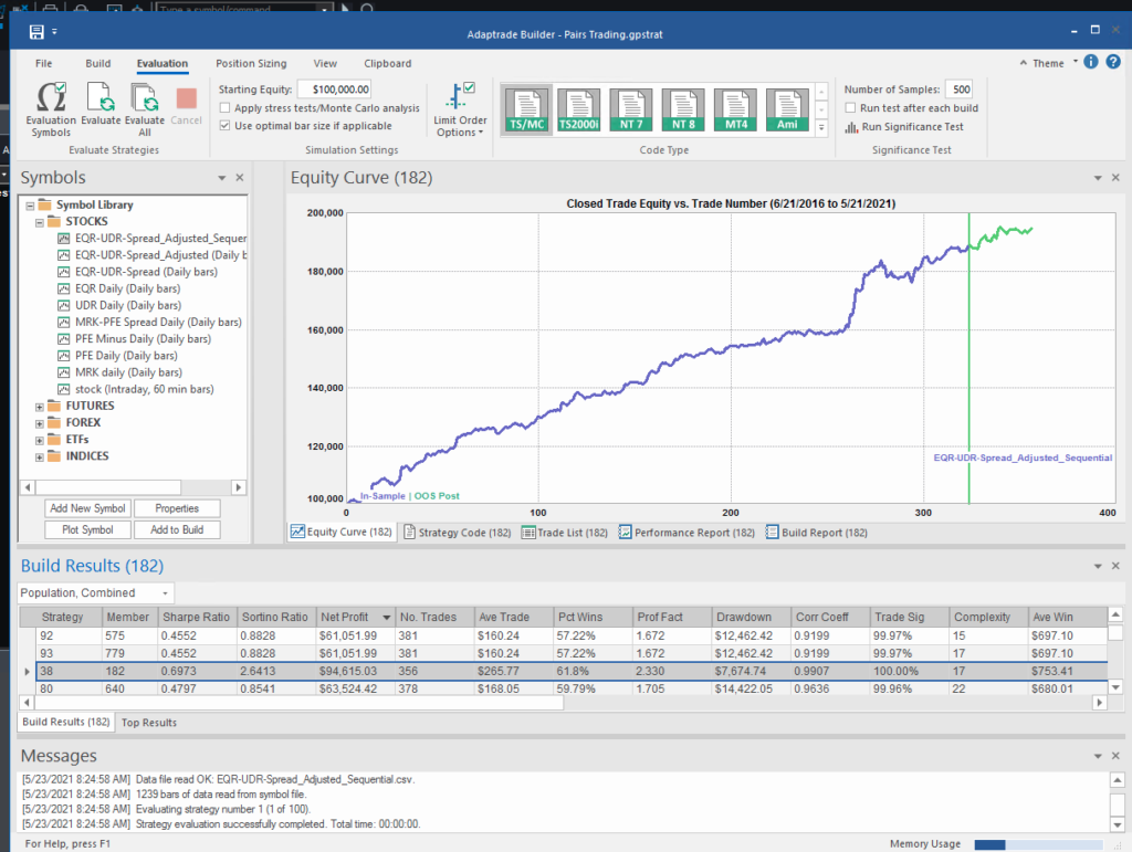
In fact this strategy has higher returns, Sharpe Ratio, Sortino Ratio and lower drawdown than many of the earlier models.
Conclusion
The purpose of this post was to show how we can combine the standard approach to statistical arbitrage, which is based on classical econometric theory, with modern machine learning algorithms, such as genetic programming. This frees us to consider a very much wider range of possible trade entry and exit strategies, beyond the rather simplistic approach adopted when pairs trading was first developed. We can deploy multiple trade entry levels and stop loss levels to manage risk, dynamically size the trade according to current market conditions and give emphasis to alternative performance characteristics such as maximum drawdown, or Sharpe or Sortino ratio, in addition to strategy profitability.
The programatic nature of the strategies developed in the way also make them very amenable to optimization, Monte Carlo simulation and stress testing.
This is but one way of adding machine learning methodologies to the mix. In a series of follow-up posts I will be looking at the role that other machine learning techniques - such as deep learning and reinforcement learning - can play in improving the performance characteristics of the classical statistical arbitrage strategy.