Half Hex Atlas
The following code is a slightly less-involved derivation of apparently the same rules seen above. (Equivalence of rule sets can be verified in practice by comparing counting functions for sufficiently long time intervals). See also: Whole Hex Rule Derivation.
star = ReIm[Exp[I 2 Pi #/3]] & /@ Range[0, 2];
ToCanonical[vec_] := Subtract[vec, Floor[Divide[vec.{1, 1, 1}, 3] ]]
NeighborLocs[or_, 1] := Map[ToCanonical[or + #] &,
Riffle[IdentityMatrix[3], RotateRight[-IdentityMatrix[3]]]]
NeighborLocs[or_, n_] := Join[NeighborLocs[or, n - 1],
Flatten[Partition[NeighborLocs[or, 1], 3, 1, 1]
/. {x_List, y_List, z_List} :> Map[
ToCanonical[or + n x + # z] &, Range[0, n - 1]], 1]]
InfM = RotateRight[{2, 0, 0}, #] & /@ Range[0, 2];
InflateRep = {T[x_, v_] :> Prepend[Join[
T[ToCanonical[InfM.x] + IdentityMatrix[3][[#]], #] & /@ Range[3],
T[ToCanonical[InfM.x] - IdentityMatrix[3][[#]], #] & /@
Range[3]],
T[ToCanonical[InfM.x], v]]};
Depict[v_, c_] := {c /. {1 -> Red, 2 -> Green, 3 -> Blue, 0 -> White},
Disk[v.star, 1/2]};
tilingData = NestList[Union[Flatten[# /. InflateRep]] &,
T[{0, 0, 0}, 1] /. InflateRep, 4];
NeighborVals[data_, or_] := With[{locs = NeighborLocs[or, 1]},
ReplaceAll[Cases[data, T[#, dir_] :> dir], {} -> {0}][[1]] & /@ locs]
GetTemplates[data_] := Union[Select[
NeighborVals[data, #[[1]] ] -> #[[2]] & /@ data,
! MemberQ[#[[1]], 0] &]]
AbsoluteTiming[
templates = GetTemplates /@ tilingData[[1 ;; 4]];
Length /@ templates;]
DepictTemplate[rule_] := Graphics[{
Depict[{0, 0, 0}, rule[[2]]],
MapThread[Depict, {NeighborLocs[{0, 0, 0}, 1], rule[[1]]}]
}, ImageSize -> 75]
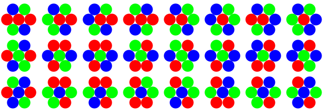
SortedInds =
Cases[Position[templates[[-1]], #], {x_, 2} :> x] & /@ Range[1, 3];
GraphicsGrid[
Partition[DepictTemplate /@ templates[[-1, Flatten[SortedInds]]],
8]];
partials[temp_] :=
ReplacePart[temp, Alternatives @@ # -> _] & /@ Subsets[Range[6]]
AllPartials =
Union[Flatten[partials /@ templates[[3, SortedInds[[#]], 1]],
1]] & /@ Range[3];
FilteredPartials = Complement[AllPartials[[#]],
Flatten[AllPartials[[Complement[Range[3], {#}]]] , 1] ] & /@
Range[3];
Subsets[Range[3], {2}] /. {{x_, y_} :>
Intersection[FilteredPartials[[x]], FilteredPartials[[y]]]};
DefiniteRules = {Alternatives @@ FilteredPartials[[1]] -> 1,
Alternatives @@ FilteredPartials[[2]] -> 2,
Alternatives @@ FilteredPartials[[3]] -> 3};
OnRules = Flatten[
Outer[RotateRight[{#2, 0, 0, 0, 0, 0}, #1] ->
RotateLeft[Range[3], #1][[1]] &, Range[0, 5], Range[3]]];
ExtRules = Join[Map[
RotateLeft[{RotateRight[Range[3], #][[1]],
RotateRight[Range[3], #][[2]], 0, 0, 0, 0}, #] ->
RotateRight[Range[3], #][[3]] &, Range[0, 5]], Map[
RotateLeft[{RotateRight[Range[3], #][[2]],
RotateRight[Range[3], #][[1]], 0, 0, 0, 0}, #] ->
RotateRight[Range[3], #][[3]] &, Range[0, 5]]];
CollideRules = Map[
RotateLeft[{RotateRight[Range[3], #][[1]], 0, 0,
RotateRight[Range[3], #][[1]], 0, 0}, #] ->
RotateRight[Range[3], #][[1]] &, Range[0, 2]];
AllRules = Join[DefiniteRules,
OnRules /. {2 -> 3, 3 -> 2},
ExtRules /. {2 -> 3, 3 -> 2},
CollideRules /. {2 -> 3, 3 -> 2}];
State0 = {{T[{0, 0, 0}, 1]}, {}};
Iterate[state_] := With[{newVerts = Complement[
Flatten[NeighborLocs[#, 1] & /@ state[[1, All, 1]], 1],
Flatten[state[[All, All, 1]], 1]]},
Flatten /@ {MapThread[
If[IntegerQ[#2], T[#1, #2], {}] &, {newVerts,
ReplaceAll[NeighborVals[Flatten[state], #],
AllRules] & /@ newVerts}], state}]
Graphics[Flatten[Nest[Iterate, State0, 4 #]] /. T -> Depict] & /@
Range[5];
GrowthData65 = NestList[Iterate, State0, 65];
Complement[Flatten[GrowthData65[[-1]]],
Nest[Flatten[# /. InflateRep] &, T[{0, 0, 0}, 1], 7]]
Out[]={}
Length[#[[1]] ] & /@ GrowthData65
%[[2 ;; -1]]/6
Flatten[Position[%, 3]]
Differences[%]
Out[]={1, 6, 12, 18, 24, 18, 42, 48, 48, 18, 42, 66, 90, 60, 120, 108, 96,
18, 42, 66, 90, 66, 162, 186, 186, 60, 138, 216, 264, 162, 276, 228,
192, 18, 42, 66, 90, 66, 162, 186, 186, 66, 162, 258, 354, 234, 474,
426, 378, 60, 138, 216, 282, 234, 528, 600, 552, 162, 366, 570, 630,
366, 588, 468, 384, 18}
Out[]={1, 2, 3, 4, 3, 7, 8, 8, 3, 7, 11, 15, 10, 20, 18, 16, 3, 7, 11, 15,
11, 27, 31, 31, 10, 23, 36, 44, 27, 46, 38, 32, 3, 7, 11, 15, 11, 27,
31, 31, 11, 27, 43, 59, 39, 79, 71, 63, 10, 23, 36, 47, 39, 88, 100,
92, 27, 61, 95, 105, 61, 98, 78, 64, 3}
Out[]={3, 5, 9, 17, 33, 65}
Out[]={2, 4, 8, 16, 32}
The last output shows log-periodicity with inflation factor
$2$, thus the C.A. does have what we called "Ulam Structure" elsewhere. For reference, the
$85$ derived rules are:
AllRules2

Out[]={
{0, 0, 0, 0, 0, 1} -> 2
{0, 0, 0, 0, 1, 0} -> 3
{0, 0, 0, 1, 0, 0} -> 1
{0, 0, 1, 0, 0, 0} -> 2
{0, 1, 0, 0, 0, 0} -> 3
{1, 0, 0, 0, 0, 0} -> 1
{0, 0, 0, 0, 0, 2} -> 2
{0, 0, 0, 0, 2, 3} -> 1
{0, 0, 0, 0, 3, 0} -> 3
{0, 0, 0, 3, 1, 0} -> 2
{0, 0, 1, 2, 0, 0} -> 3
{0, 0, 2, 0, 0, 0} -> 2
{0, 2, 3, 0, 0, 0} -> 1
{0, 3, 0, 0, 0, 0} -> 3
{2, 0, 0, 0, 0, 1} -> 3
{3, 1, 0, 0, 0, 0} -> 2
{0, 0, 0, 0, 1, 3} -> 2
{0, 0, 0, 0, 2, 1} -> 3
{0, 0, 0, 2, 1, 0} -> 3
{0, 0, 0, 3, 2, 0} -> 1
{0, 0, 1, 3, 0, 0} -> 2
{0, 0, 3, 2, 0, 0} -> 1
{0, 1, 3, 0, 0, 0} -> 2
{0, 2, 1, 0, 0, 0} -> 3
{2, 0, 0, 0, 0, 3} -> 1
{2, 1, 0, 0, 0, 0} -> 3
{3, 0, 0, 0, 0, 1} -> 2
{3, 2, 0, 0, 0, 0} -> 1
{0, 0, 0, 0, 3, 2} -> 1
{0, 0, 0, 1, 3, 0} -> 2
{0, 0, 2, 1, 0, 0} -> 3
{0, 3, 2, 0, 0, 0} -> 1
{1, 0, 0, 0, 0, 2} -> 3
{1, 3, 0, 0, 0, 0} -> 2
{0, 0, 0, 2, 2, 3} -> 1
{0, 0, 0, 3, 1, 1} -> 2
{0, 0, 1, 2, 2, 0} -> 3
{0, 0, 3, 3, 1, 0} -> 2
{0, 1, 1, 2, 0, 0} -> 3
{0, 2, 3, 3, 0, 0} -> 1
{2, 0, 0, 0, 1, 1} -> 3
{2, 2, 0, 0, 0, 1} -> 3
{2, 2, 3, 0, 0, 0} -> 1
{3, 0, 0, 0, 2, 3} -> 1
{3, 1, 0, 0, 0, 3} -> 2
{3, 1, 1, 0, 0, 0} -> 2
{0, 0, 1, 3, 1, 3} -> 2
{0, 2, 1, 2, 1, 0} -> 3
{2, 0, 0, 3, 2, 3} -> 1
{2, 1, 0, 0, 2, 1} -> 3
{3, 1, 3, 0, 0, 1} -> 2
{3, 2, 3, 2, 0, 0} -> 1
{0, 0, 0, 2, 1, 1} -> 3
{0, 0, 0, 2, 2, 1} -> 3
{0, 0, 3, 2, 2, 0} -> 1
{0, 0, 3, 3, 2, 0} -> 1
{0, 1, 1, 3, 0, 0} -> 2
{0, 1, 3, 3, 0, 0} -> 2
{2, 1, 1, 0, 0, 0} -> 3
{2, 2, 0, 0, 0, 3} -> 1
{2, 2, 1, 0, 0, 0} -> 3
{3, 0, 0, 0, 1, 1} -> 2
{3, 0, 0, 0, 1, 3} -> 2
{3, 2, 0, 0, 0, 3} -> 1
{0, 0, 3, 3, 1, 1} -> 2
{0, 1, 1, 2, 2, 0} -> 3
{2, 2, 0, 0, 1, 1} -> 3
{2, 2, 3, 3, 0, 0} -> 1
{3, 0, 0, 2, 2, 3} -> 1
{3, 1, 1, 0, 0, 3} -> 2
{0, 0, 1, 2, 2, 1} -> 3
{0, 0, 2, 0, 0, 2} -> 2
{0, 0, 3, 2, 2, 3} -> 1
{0, 1, 3, 3, 1, 0} -> 2
{0, 2, 3, 3, 2, 0} -> 1
{0, 3, 0, 0, 3, 0} -> 3
{1, 0, 0, 1, 0, 0} -> 1
{2, 0, 0, 2, 1, 1} -> 3
{2, 1, 1, 2, 0, 0} -> 3
{2, 2, 1, 0, 0, 1} -> 3
{2, 2, 3, 0, 0, 3} -> 1
{3, 0, 0, 3, 1, 1} -> 2
{3, 1, 0, 0, 1, 3} -> 2
{3, 1, 1, 3, 0, 0} -> 2
{3, 2, 0, 0, 2, 3} -> 1
}


