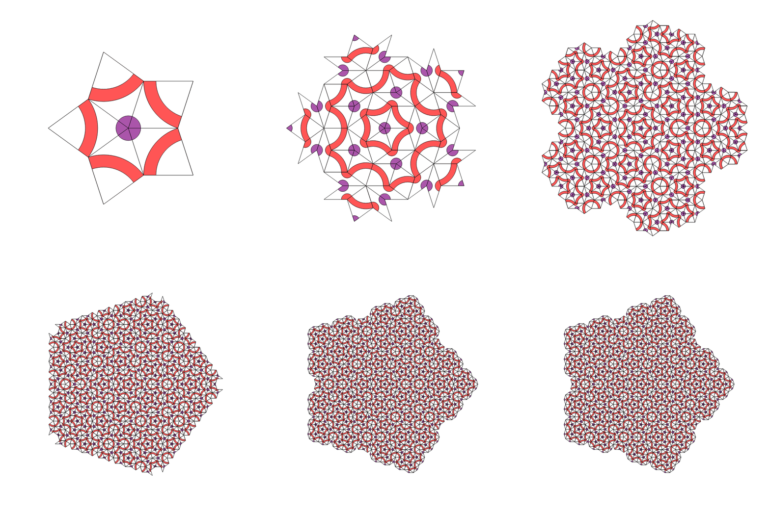
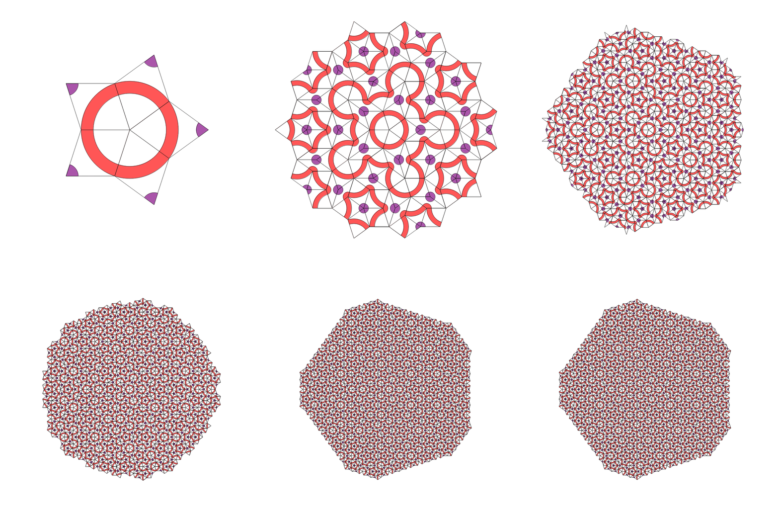
In two previous posts on plane patterns, we discuss the relation between substitution systems, cellular automata and template atlases. Another plane pattern, the Penrose tiling, presents considerable difficulties in the form of non-crystallographic symmetry. Most people wouldn't bother to try and find a growth function, but we have two reasons to do just that. First, growth functions introduce a time variable, so provide a way from mathematical structure into physical process, thus toward the realm of quasicrystals. Second, perhaps more importantly, we would like to spend some of our limited time on this earth in the pursuit of pure beauty (even though pursuit of pure beauty might also be pursuit of total misery).
We need some functions to draw the actual tiles. To make the growth process easier, we put control points on every vertex, and allow for ten distinct orientations:
DepictThin[or_, v_, r_] := With[{verts = {{0, 0},
     {Cos[2 r Pi/10], Sin[2 r Pi/10]},
     {Cos[2 r Pi/10], Sin[2 r Pi/10]}
      + {Cos[2 (r - 1) Pi/10], Sin[2 (r - 1) Pi/10]},
     {Cos[2 (r - 1) Pi/10], Sin[2 (r - 1) Pi/10]}}},
  {White, Polygon[Expand@Plus[or, #, Part[-verts, v]] & /@ verts],
   Lighter@Red,
   Disk[or + Part[-verts, v] + verts[[2]],
    1/4, {2 (r - 1) Pi/10, 2 (r - 5) Pi/10}],
   Lighter@Purple,
   Disk[or + Part[-verts, v] + verts[[4]],
    1/4, {2 (r) Pi/10, 2 (r + 4) Pi/10}]}]

DepictFat[or_, v_, r_] := With[{verts = {{0, 0},
     {Cos[2 r Pi/10], Sin[2 r Pi/10]},
     {Cos[2 r Pi/10], Sin[2 r Pi/10]}
      + {Cos[2 (r - 2) Pi/10], Sin[2 (r - 2) Pi/10]},
     {Cos[2 (r - 2) Pi/10], Sin[2 (r - 2) Pi/10]}}},
  {White, Polygon[Expand@Plus[or, #, Part[-verts, v]] & /@ verts],
   Lighter@Purple, Disk[or + Part[-verts, v] + verts[[1]],
    1/4, {2 (r) Pi/10, 2 (r - 2) Pi/10}],
   Lighter@Red, Disk[or + Part[-verts, v] + verts[[3]],
    1, {2 (r + 5) Pi/10, 2 (r + 3) Pi/10}],
   White, Disk[or + Part[-verts, v] + verts[[3]],
    3/4, {2 (r + 5) Pi/10, 2 (r + 3) Pi/10}]}]
DepictRule = {TF -> DepictFat, TT -> DepictThin};
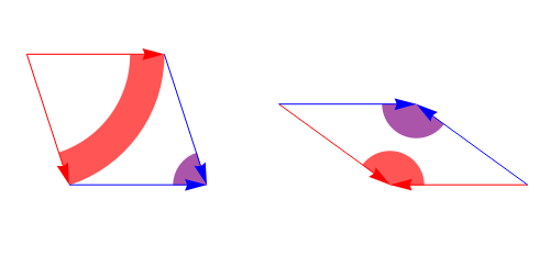
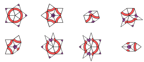
The one tile is usually called fat and the other thin. These tiles have matching rules, so they can only group around a vertex in one of eight legal vertex figures (in this case, vertex figures are essentially the same thing as what NKS calls templates). The atlas of all possible vertex figures is written out fully as:
Stars = Function[{off}, TF[{0, 0}, 1, 2 # - off] & /@ Range[5]] /@ {0,1};
Suns = Function[{off}, TF[{0, 0}, 3, 2 # - off] & /@ Range[5]] /@ {0, 1};
FHexes = Map[{TF[{0, 0}, 2, Mod[2 + #, 10]],
     TF[{0, 0}, 4, Mod[4 + #, 10]],
     TT[{0, 0}, 2, Mod[5 + #, 10]]} &, Range[10]];
Crowns = Map[{TF[{0, 0}, 4, Mod[2 + #, 10]],
     TF[{0, 0}, 2, Mod[4 + #, 10]],
     TT[{0, 0}, 3, Mod[4 + #, 10]], TF[{0, 0}, 3, Mod[3 + #, 10]],
     TT[{0, 0}, 1, Mod[6 + #, 10]]} &, Range[10]];
Boats = Map[{TF[{0, 0}, 1, Mod[6 + #, 10]],
     TF[{0, 0}, 1, Mod[4 + #, 10]],
     TF[{0, 0}, 1, Mod[2 + #, 10]], TT[{0, 0}, 4, Mod[6 + #, 10]]} &,
   Range[10]];
Splits = Map[{TF[{0, 0}, 3, Mod[#, 10]], TF[{0, 0}, 3, Mod[2 + #, 10]],
     TF[{0, 0}, 3, Mod[4 + #, 10]], TF[{0, 0}, 3, Mod[6 + #, 10]],
     TT[{0, 0}, 3, Mod[7 + #, 10]], TT[{0, 0}, 1, Mod[3 + #, 10]]} &,
   Range[10]];
Wings = Map[{TT[{0, 0}, 1, Mod[7 + #, 10]],
     TT[{0, 0}, 3, Mod[1 + #, 10]],
     TF[{0, 0}, 3, Mod[#, 10]],
     TT[{0, 0}, 1, Mod[3 + #, 10]], TT[{0, 0}, 3, Mod[7 + #, 10]],
     TF[{0, 0}, 3, Mod[6 + #, 10]], TF[{0, 0}, 3, Mod[4 + #, 10]]
     } &, Range[10]];
THexes = Map[{TT[{0, 0}, 4, Mod[#, 10]], TT[{0, 0}, 4, Mod[4 + #, 10]],
     TF[{0, 0}, 1, Mod[#, 10]]} &, Range[10]];
AllFigures = List[Suns, Stars, FHexes, Crowns, Boats, Splits, Wings, THexes];

Partition[Map[Graphics[{EdgeForm[Black], # /. DepictRule},
     PlotRange -> {{-2, 2}, {-2, 2}}, ImageSize -> 100] &,
   AllFigures[[All, 1]], {1}], 4] // TableForm
Assume that we have a partially complete tiling and would like to add more tiles along the boundary. To do so, we need to know: which partial configurations have a unique completion? To answer this question, we simply calculate all possible partial configurations and notice when some are unique, while others project down from multiple vertex figures. The combinatorics can be programmed, so it ultimately requires very little thought:
FatEdges[or_, v_, r_] := With[{verts = {{0, 0},
     {Cos[2 r Pi/10], Sin[2 r Pi/10]},
     {Cos[2 r Pi/10], Sin[2 r Pi/10]}
      + {Cos[2 (r - 2) Pi/10], Sin[2 (r - 2) Pi/10]},
     {Cos[2 (r - 2) Pi/10], Sin[2 (r - 2) Pi/10]}}},
  Function[{verts},
    {FC[verts[[1]], Mod[r, 10]], TC[verts[[2]], Mod[r + 5, 10]],
     FC[verts[[1]], Mod[r - 2, 10]], TC[verts[[4]], Mod[r + 3, 10]],
     FR[verts[[4]], Mod[r, 10]], TR[verts[[3]], Mod[r + 5, 10]],
     FR[verts[[2]], Mod[r - 2, 10]], TR[verts[[3]], Mod[r + 3, 10]]}
    ][Expand@Plus[or, #, Part[-verts, v]] & /@ verts]]

ThinEdges[or_, v_, r_] := With[{verts = {{0, 0},
     {Cos[2 r Pi/10], Sin[2 r Pi/10]},
     {Cos[2 r Pi/10], Sin[2 r Pi/10]}
      + {Cos[2 (r - 1) Pi/10], Sin[2 (r - 1) Pi/10]},
     {Cos[2 (r - 1) Pi/10], Sin[2 (r - 1) Pi/10]}}},
  Function[{verts},
    {TR[verts[[1]], Mod[r, 10]], FR[verts[[2]], Mod[r + 5, 10]],
     TC[verts[[1]], Mod[r - 1, 10]], FC[verts[[4]], Mod[r + 4, 10]],
     FC[verts[[4]], Mod[r, 10]], TC[verts[[3]], Mod[r + 5, 10]],
     FR[verts[[2]], Mod[r - 1, 10]], TR[verts[[3]], Mod[r + 4, 10]]}
    ][Expand@Plus[or, #, Part[-verts, v]] & /@ verts]]

EdgesRule = {TF -> FatEdges, TT -> ThinEdges};

ProjectRules[figure_] := Rule @@ # & /@ Map[List[ Sort[
  Cases[figure[[1 ;; #]] /. EdgesRule, xF_[{0, 0}, yr_] :> xF[yr],
    Infinity]],
 figure[[#1 + 1 ;; -1]] ] &, Range[2, Length[figure] - 1]]

CompletionMap = Flatten[Map[Function[{rot}, ProjectRules[RotateRight[#, rot]]
     ] /@ Range[Length[#]] &, #] & /@ AllFigures];

UniqueCompletion = Cases[Tally[CompletionMap[[All, 1]]], {x_, 1} :> x];

UniqueMap = MapThread[ Rule, {UniqueCompletion, UniqueCompletion /. CompletionMap}];

AddRep[or_] := ReplaceAll[UniqueMap, {0, 0} -> or]
To see what we've done here (quite a lot by data structure and mapping), let's add another intermediary depiction function. There are $410$ total rules in AddRep, so we will only plot a random sample of 16:
DepictAddRule[rule_] := Show[Reverse[Map[Graphics[{EdgeForm[Thin],
       Arrowheads[.1], Thick, # /. DepictRule},
      ImageSize -> 150, PlotRange -> {{-2, 2}, {-2, 2}}] &, rule /.
      Rule -> List /. {FR[r_] :> {Red,
        Arrow[{{Cos[r Pi/5], Sin[r Pi/5]}, {0, 0}}]},
      FC[r_] :> {Blue, Arrow[{{Cos[r Pi/5], Sin[r Pi/5]}, {0, 0}}]},
      TR[r_] :> {Red,
        Arrow[Reverse@{{Cos[r Pi/5], Sin[r Pi/5]}, {0, 0}}]},
      TC[r_] :> {Blue,
        Arrow[Reverse@{{Cos[r Pi/5], Sin[r Pi/5]}, {0, 0}}]}}, 1]]]

Partition[DepictAddRule /@ RandomSample[AddRep[{0, 0}], 16],
  4] // TableForm
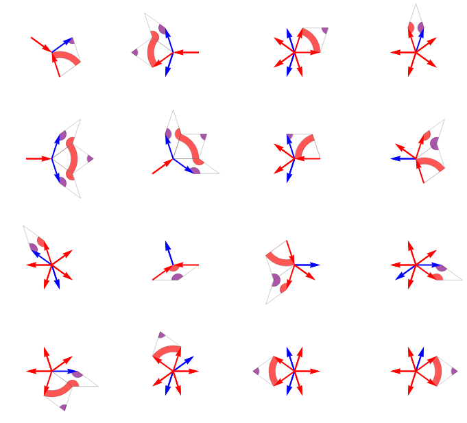
Basically, each image says that if we find this particular configuration of edge vectors in a partially complete tiling, then we should add one or more tiles, as depicted, to complete the figure. This is all good, but if we try to use only these $410$ rules, we quickly meet ambiguous conditions where we must choose one of two alternatives:
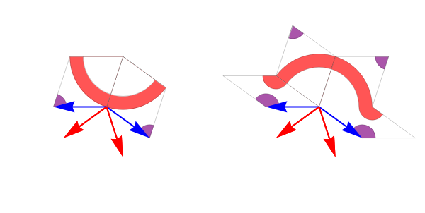
In another beautiful apparition of parity symmetry, it turns out the first alternative is better for growing the Night configuration, while the second is better for Day. All that's left is to define iterators and axioms as follows:
StarFailSafe[or_] := Join[
  Sort[{TC[Mod[2 + #, 10]], TC[Mod[6 + #, 10]], TR[Mod[3 + #, 10]],
       TR[Mod[3 + #, 10]], TR[Mod[5 + #, 10]],
       TR[Mod[5 + #, 10]]}] -> {TF[or, 2, # + 1],
      TF[or, 4, # - 1]} & /@ Range[10]]

SunFailSafe[or_] := Join[Sort[
      {TC[Mod[2 + #, 10]], TC[Mod[6 + #, 10]], TR[Mod[3 + #, 10]],
       TR[Mod[3 + #, 10]], TR[Mod[5 + #, 10]],
       TR[Mod[5 + #, 10]]}] -> {TF[or, 3, # + 6], TF[or, 3, # + 4],
      TT[or, 1, # - 3], TT[or, 3, # + 7]} & /@ Range[10],
  Sort[{TC[Mod[# + 1, 10]], TC[Mod[# + 1, 10]], TR[Mod[#, 10]],
       TR[Mod[#, 10]],
       TR[Mod[# + 2, 10]], TR[Mod[# + 2, 10]], TR[Mod[# + 4, 10]],
       TR[Mod[# + 8, 10]]
       }] -> {TF[or, 3, Mod[1 + #, 10]],
      TF[or, 3, Mod[3 + #, 10]]} & /@ Range[10]]

CompleteFigures =   Map[Sort[Cases[# /. EdgesRule, xF_[{0, 0}, yr_] :> xF[yr],
      Infinity]] &,   Flatten[AllFigures, 1]];

 IterateSunFS[state_, comp_] := With[{VertexFigures = Function[{edges},
      V[#, Sort[Cases[edges, x_[#, y_] :> x[y]]]] & /@ (
        Complement[Union[edges[[All, 1]]], comp])][
     Flatten[Union[state /. EdgesRule]]]},
  {Join[state, If[Length[#] == 0, Print["^"];
       With[{hits =
          Cases[VertexFigures /.
            V[or_, edges_] :> (edges /. SunFailSafe[or]),
           TT[__] | TF[__], Infinity]},
        Sow[hits]; hits], #] &@
     Cases[VertexFigures /. V[or_, edges_] :> (edges /. AddRep[or]),
      TT[__] | TF[__], Infinity]],
   Join[comp,
    Cases[VertexFigures,
     V[x_, Alternatives @@ CompleteFigures] :> x]]}]

IterateStarFS[state_, comp_] := With[{VertexFigures = Function[{edges},
      V[#, Sort[Cases[edges, x_[#, y_] :> x[y]]]] & /@ (
        Complement[Union[edges[[All, 1]]], comp])][
     Flatten[Union[state /. EdgesRule]]]},
  {Join[state, If[Length[#] == 0, Print["^"];
       With[{hits =
          Cases[VertexFigures /.
            V[or_, edges_] :> (edges /. StarFailSafe[or]),
           TT[__] | TF[__], Infinity]},
        Sow[hits]; hits], #] &@
     Cases[VertexFigures /. V[or_, edges_] :> (edges /. AddRep[or]),
      TT[__] | TF[__], Infinity]],
   Join[comp,
    Cases[VertexFigures,
     V[x_, Alternatives @@ CompleteFigures] :> x]]}]

AxiomA = TF[{0, 0}, 1, 2 #] & /@ Range[5];
StateA1 = {AxiomA, {{0, 0}}};
AxiomB = TF[{0, 0}, 3, 2 #] & /@ Range[5];
StateB1 = {AxiomB, {{0, 0}}};
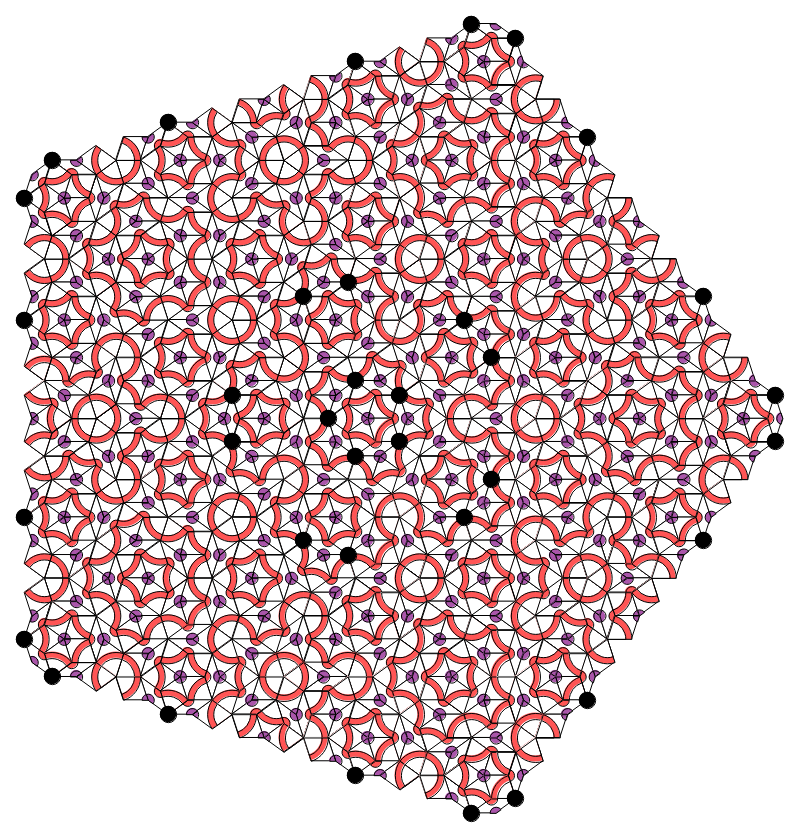
Now we can generate successive configurations and make a plot of where we were forced to make an arbitrary choice to continue growing the tiling. For the night configuration, we have, after about $35$ iterations:
AbsoluteTiming[ AData = Reap[NestList[IterateStarFS @@ # &, StateA1, 40]];]
Graphics[{EdgeForm[Black], AData[[1, -5, 1]] /. DepictRule,
  Map[Disk[#, 1/3] &,   Union[Flatten[AData[[2, 1, All, All, 1]], 1]]]}, ImageSize -> 800]
And for the Day configuration, we have, after about $45$ iterations:
AbsoluteTiming[ data = Reap[NestList[IterateSunFS @@ # &, StateB1, 50]];]

Graphics[{EdgeForm[Black], data[[1, -5, 1]] /. DepictRule,
  Map[Disk[#, 1/3] &,
   Union[Flatten[data[[2, 1, All, All, 1]], 1]]]}, ImageSize -> 800]
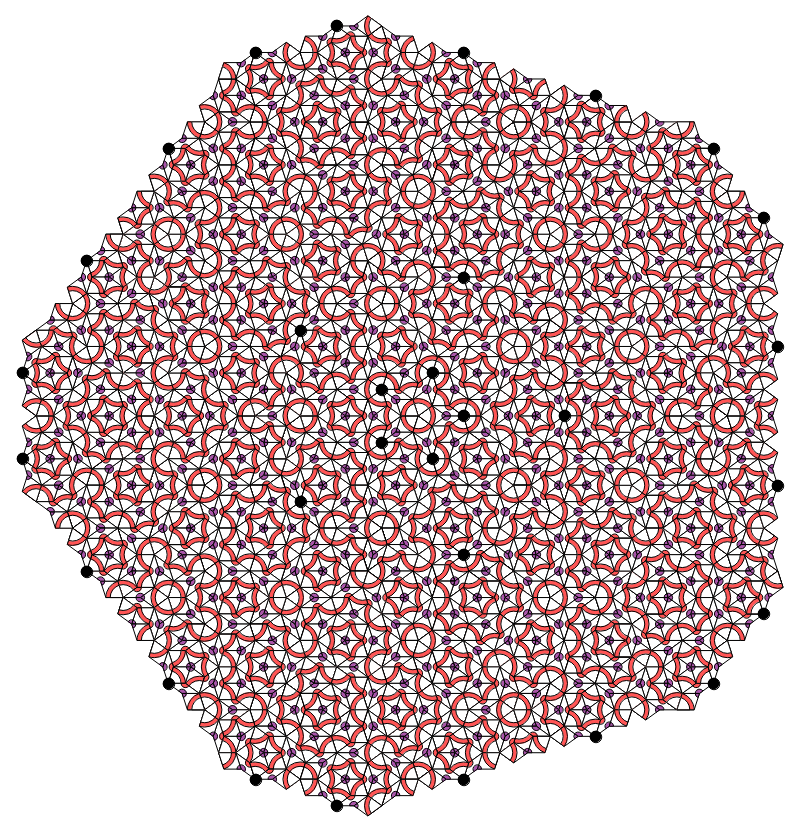
Using the same code, we can easily check both patterns up to $t\approx 150$, which gets us past the fourth or fifth wave / corona, in terms of light-red loops drawn around the pattern center. This very strongly suggests that the algorithm as presented here will grow patterns indefinitely. However, a little more work remains to be done to make the algorithm a proper Cellular Automaton algorithm. This can likely be accomplished by adding an extra binary variable at all binary-ambiguous vertices. This project we leave for another day...