After g.t.
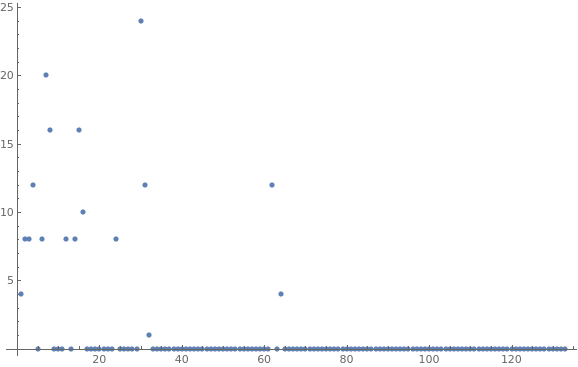
$20$ minutes, the computer finally produced the following graph, which counts new rules needed as a function of time:
Length /@ ReducedCodeData2
Total[%]
ListPlot[%%]

Out[]= {4, 8, 8, 12, 0, 8, 20, 16, 0, 0, 0, 8, 0, 8, 16, 10, 0, 0, 0, 0, 0,
0, 0, 8, 0, 0, 0, 0, 0, 24, 12, 1, 0, 0, 0, 0, 0, 0, 0, 0, 0, 0, 0,
0, 0, 0, 0, 0, 0, 0, 0, 0, 0, 0, 0, 0, 0, 0, 0, 0, 0, 12, 0, 4, 0, 0,
0, 0, 0, 0, 0, 0, 0, 0, 0, 0, 0, 0, 0, 0, 0, 0, 0, 0, 0, 0, 0, 0, 0,
0, 0, 0, 0, 0, 0, 0, 0, 0, 0, 0, 0, 0, 0, 0, 0, 0, 0, 0, 0, 0, 0, 0,
0, 0, 0, 0, 0, 0, 0, 0, 0, 0, 0, 0, 0, 0, 0, 0, 0, 0, 0, 0, 0}

Out[]=179
When running the C.A. a small time savings (l.t. factor 2) can be found by using only the 179 rules. For reference those 179 rules are printed off as:
AllRules2

Out[156]=

 {
{0, 0, 0, 1, 0, 0, 0, 0} -> 3
{0, 0, 0, 3, 0, 0, 0, 0} -> 3
{0, 0, 0, 5, 0, 0, 0, 0} -> 5
{0, 0, 0, 5, 0, 0, 0, 1} -> 5
{0, 0, 0, 5, 0, 0, 1, 0} -> 5
{0, 0, 0, 5, 0, 1, 0, 0} -> 5
{0, 0, 0, 5, 0, 1, 0, 1} -> 5
{0, 0, 0, 5, 0, 1, 1, 0} -> 5
{0, 0, 0, 5, 1, 0, 0, 0} -> 5
{0, 0, 0, 5, 1, 0, 0, 1} -> 5
{0, 0, 0, 5, 1, 0, 1, 0} -> 5
{0, 0, 0, 5, 1, 1, 0, 0} -> 5
{0, 0, 0, 5, 1, 1, 0, 1} -> 5
{0, 0, 0, 5, 1, 1, 1, 0} -> 5
{0, 0, 1, 0, 0, 0, 0, 0} -> 2
{0, 0, 1, 2, 0, 0, 2, 0} -> 5
{0, 0, 1, 4, 0, 0, 4, 0} -> 5
{0, 0, 2, 0, 0, 0, 0, 0} -> 2
{0, 0, 3, 1, 0, 0, 3, 0} -> 4
{0, 0, 3, 2, 0, 0, 1, 0} -> 1
{0, 0, 3, 4, 0, 0, 3, 0} -> 1
{0, 0, 4, 0, 0, 0, 0, 0} -> 4
{0, 0, 4, 0, 0, 0, 0, 1} -> 4
{0, 0, 4, 0, 0, 0, 1, 0} -> 4
{0, 0, 4, 0, 0, 0, 1, 1} -> 4
{0, 0, 4, 0, 0, 1, 0, 0} -> 4
{0, 0, 4, 0, 0, 1, 0, 1} -> 4
{0, 0, 4, 0, 1, 0, 0, 0} -> 4
{0, 0, 4, 0, 1, 0, 0, 1} -> 4
{0, 0, 4, 0, 1, 0, 1, 0} -> 4
{0, 0, 4, 0, 1, 0, 1, 1} -> 4
{0, 0, 4, 0, 1, 1, 0, 0} -> 4
{0, 0, 4, 0, 1, 1, 0, 1} -> 4
{0, 0, 4, 5, 0, 0, 0, 0} -> 1
{0, 0, 4, 5, 0, 0, 1, 0} -> 1
{0, 0, 5, 1, 0, 0, 5, 0} -> 4
{0, 0, 5, 2, 0, 0, 2, 0} -> 1
{0, 0, 5, 4, 0, 0, 4, 0} -> 1
{0, 0, 5, 4, 0, 0, 4, 1} -> 1
{0, 0, 5, 4, 0, 0, 5, 0} -> 1
{0, 0, 5, 4, 0, 0, 5, 1} -> 1
{0, 0, 5, 4, 0, 1, 4, 0} -> 1
{0, 0, 5, 4, 0, 1, 5, 0} -> 1
{0, 0, 5, 4, 1, 0, 4, 0} -> 1
{0, 0, 5, 4, 1, 0, 5, 0} -> 1
{0, 1, 0, 0, 0, 0, 0, 0} -> 5
{0, 1, 1, 4, 0, 4, 4, 0} -> 5
{0, 1, 1, 5, 0, 4, 0, 0} -> 5
{0, 1, 3, 0, 0, 3, 0, 0} -> 4
{0, 1, 5, 0, 0, 5, 0, 0} -> 4
{0, 2, 1, 0, 0, 2, 0, 0} -> 3
{0, 2, 3, 0, 0, 2, 0, 0} -> 1
{0, 2, 5, 0, 0, 1, 0, 0} -> 1
{0, 3, 0, 0, 0, 0, 0, 0} -> 3
{0, 3, 0, 0, 0, 0, 0, 1} -> 3
{0, 3, 0, 0, 0, 0, 1, 0} -> 3
{0, 3, 0, 0, 0, 0, 1, 1} -> 3
{0, 3, 0, 0, 0, 1, 0, 0} -> 3
{0, 3, 0, 0, 0, 1, 0, 1} -> 3
{0, 3, 0, 0, 0, 1, 1, 0} -> 3
{0, 3, 0, 0, 0, 1, 1, 1} -> 3
{0, 3, 0, 0, 1, 0, 0, 0} -> 3
{0, 3, 0, 0, 1, 0, 0, 1} -> 3
{0, 3, 0, 0, 1, 0, 1, 0} -> 3
{0, 3, 0, 0, 1, 0, 1, 1} -> 3
{0, 3, 1, 1, 0, 0, 4, 0} -> 3
{0, 3, 4, 0, 0, 0, 0, 0} -> 1
{0, 3, 4, 0, 0, 1, 0, 0} -> 1
{0, 4, 1, 0, 0, 4, 0, 0} -> 3
{0, 4, 1, 1, 0, 4, 4, 0} -> 3
{0, 4, 3, 0, 0, 3, 0, 0} -> 1
{0, 4, 3, 0, 0, 3, 0, 1} -> 1
{0, 4, 3, 0, 0, 3, 1, 0} -> 1
{0, 4, 3, 0, 0, 4, 0, 0} -> 1
{0, 4, 3, 0, 0, 4, 0, 1} -> 1
{0, 4, 3, 0, 0, 4, 1, 0} -> 1
{0, 4, 3, 0, 1, 3, 0, 0} -> 1
{0, 4, 3, 0, 1, 4, 0, 0} -> 1
{0, 4, 5, 0, 0, 5, 0, 0} -> 1
{0, 5, 0, 0, 0, 0, 0, 0} -> 5
{1, 0, 0, 0, 0, 0, 0, 0} -> 4
{1, 0, 0, 2, 0, 0, 0, 2} -> 5
{1, 0, 0, 4, 0, 0, 0, 4} -> 5
{1, 0, 4, 1, 0, 0, 0, 5} -> 4
{1, 0, 5, 1, 0, 0, 5, 5} -> 4
{1, 1, 0, 2, 2, 0, 0, 2} -> 5
{1, 1, 0, 5, 2, 0, 0, 0} -> 5
{1, 1, 1, 2, 0, 4, 0, 2} -> 5
{1, 1, 1, 2, 2, 4, 0, 2} -> 5
{1, 1, 1, 4, 2, 0, 4, 0} -> 5
{1, 1, 1, 4, 2, 4, 4, 0} -> 5
{1, 1, 1, 5, 2, 4, 0, 0} -> 5
{1, 1, 3, 0, 3, 3, 0, 0} -> 4
{1, 1, 3, 1, 0, 3, 0, 5} -> 4
{1, 1, 3, 1, 3, 3, 0, 5} -> 4
{1, 1, 4, 0, 3, 0, 0, 0} -> 4
{1, 1, 4, 1, 3, 0, 0, 5} -> 4
{1, 1, 5, 1, 3, 0, 5, 0} -> 4
{1, 1, 5, 1, 3, 0, 5, 5} -> 4
{1, 2, 0, 0, 2, 0, 0, 0} -> 3
{1, 2, 0, 1, 2, 0, 0, 2} -> 3
{1, 2, 1, 1, 2, 0, 4, 0} -> 3
{1, 2, 1, 1, 2, 0, 4, 2} -> 3
{1, 3, 0, 1, 0, 0, 0, 2} -> 3
{1, 3, 1, 1, 0, 0, 4, 2} -> 3
{1, 4, 0, 0, 4, 0, 0, 0} -> 3
{1, 4, 1, 1, 0, 4, 0, 2} -> 3
{1, 4, 1, 1, 0, 4, 4, 2} -> 3
{2, 0, 0, 0, 0, 0, 0, 0} -> 2
{2, 0, 0, 0, 0, 0, 0, 1} -> 2
{2, 0, 0, 0, 0, 0, 1, 0} -> 2
{2, 0, 0, 0, 0, 0, 1, 1} -> 2
{2, 0, 0, 0, 0, 1, 0, 0} -> 2
{2, 0, 0, 0, 0, 1, 0, 1} -> 2
{2, 0, 0, 0, 0, 1, 1, 0} -> 2
{2, 0, 0, 0, 0, 1, 1, 1} -> 2
{2, 0, 0, 0, 1, 0, 0, 0} -> 2
{2, 0, 0, 0, 1, 0, 1, 0} -> 2
{2, 0, 0, 0, 1, 1, 0, 0} -> 2
{2, 0, 0, 0, 1, 1, 1, 0} -> 2
{2, 0, 0, 5, 0, 0, 0, 0} -> 1
{2, 0, 0, 5, 0, 0, 0, 1} -> 1
{2, 0, 1, 1, 0, 0, 5, 0} -> 2
{2, 1, 1, 0, 0, 3, 0, 0} -> 2
{2, 1, 1, 1, 0, 3, 5, 0} -> 2
{2, 3, 0, 0, 0, 0, 0, 0} -> 1
{2, 3, 0, 0, 1, 0, 0, 0} -> 1
{2, 3, 4, 5, 0, 0, 0, 0} -> 1
{2, 3, 4, 5, 0, 1, 0, 1} -> 1
{2, 3, 4, 5, 1, 0, 1, 0} -> 1
{3, 0, 0, 1, 0, 0, 0, 3} -> 2
{3, 0, 0, 2, 0, 0, 0, 3} -> 1
{3, 0, 0, 4, 0, 0, 0, 1} -> 1
{3, 1, 0, 0, 3, 0, 0, 0} -> 2
{3, 1, 1, 0, 3, 3, 0, 0} -> 2
{3, 1, 1, 1, 3, 0, 5, 0} -> 2
{3, 1, 1, 1, 3, 3, 5, 0} -> 2
{3, 2, 0, 0, 2, 0, 0, 0} -> 1
{3, 2, 0, 0, 2, 0, 0, 1} -> 1
{3, 2, 0, 0, 2, 0, 1, 0} -> 1
{3, 2, 0, 0, 2, 1, 0, 0} -> 1
{3, 2, 0, 0, 3, 0, 0, 0} -> 1
{3, 2, 0, 0, 3, 0, 0, 1} -> 1
{3, 2, 0, 0, 3, 0, 1, 0} -> 1
{3, 2, 0, 0, 3, 1, 0, 0} -> 1
{3, 2, 5, 4, 2, 0, 5, 0} -> 1
{3, 2, 5, 4, 2, 0, 5, 1} -> 1
{3, 2, 5, 4, 2, 1, 5, 0} -> 1
{3, 2, 5, 4, 2, 1, 5, 1} -> 1
{3, 2, 5, 4, 3, 0, 4, 0} -> 1
{3, 2, 5, 4, 3, 0, 4, 1} -> 1
{3, 2, 5, 4, 3, 1, 4, 0} -> 1
{3, 2, 5, 4, 3, 1, 4, 1} -> 1
{3, 4, 0, 0, 4, 0, 0, 0} -> 1
{4, 0, 0, 0, 0, 0, 0, 0} -> 4
{5, 0, 0, 1, 0, 0, 0, 5} -> 2
{5, 0, 0, 2, 0, 0, 0, 2} -> 1
{5, 0, 0, 2, 0, 0, 0, 5} -> 1
{5, 0, 0, 2, 0, 0, 1, 2} -> 1
{5, 0, 0, 2, 0, 0, 1, 5} -> 1
{5, 0, 0, 2, 0, 1, 0, 2} -> 1
{5, 0, 0, 2, 0, 1, 0, 5} -> 1
{5, 0, 0, 2, 1, 0, 0, 2} -> 1
{5, 0, 0, 2, 1, 0, 0, 5} -> 1
{5, 0, 0, 4, 0, 0, 0, 4} -> 1
{5, 0, 1, 1, 0, 0, 5, 5} -> 2
{5, 1, 0, 0, 5, 0, 0, 0} -> 2
{5, 1, 1, 1, 0, 3, 0, 5} -> 2
{5, 1, 1, 1, 0, 3, 5, 5} -> 2
{5, 2, 0, 0, 5, 0, 0, 0} -> 1
{5, 4, 0, 0, 1, 0, 0, 0} -> 1
{5, 4, 3, 2, 0, 3, 0, 2} -> 1
{5, 4, 3, 2, 0, 3, 1, 2} -> 1
{5, 4, 3, 2, 0, 4, 0, 5} -> 1
{5, 4, 3, 2, 0, 4, 1, 5} -> 1
{5, 4, 3, 2, 1, 3, 0, 2} -> 1
{5, 4, 3, 2, 1, 3, 1, 2} -> 1
{5, 4, 3, 2, 1, 4, 0, 5} -> 1
{5, 4, 3, 2, 1, 4, 1, 5} -> 1
}
As indicated by the graph above, we strongly suspect these are the only rules need to infinity.


