Firstly, the Mathematica code is given as
A = -2/3000;
F = (7 Sinh[\[Xi] - 0.3 t])/(30 Cosh[\[Xi] - 0.3 t]) - (
23 Sinh[\[Xi] - 0.3 t])/(60 (Cosh[\[Xi] - 0.3 t])^3) + (
7 Sinh[\[Xi] - 0.1 t])/(15 Cosh[\[Xi] - 0.1 t]) - (
23 Sinh[\[Xi] - 0.1 t])/(30 (Cosh[\[Xi] - 0.1 t])^3) - (
7 Sinh[\[Xi] + 0.1 t])/(15 Cosh[\[Xi] + 0.1 t]) + (
23 Sinh[\[Xi] + 0.1 t])/(30 (Cosh[\[Xi] + 0.1 t])^3) + 10;
FX = 0.3 (Sech[\[Xi] - 0.3 t])^2 + 0.5 (Sech[\[Xi] - 0.1 t])^2 -
0.8 (Sech[\[Xi] + 0.1 t])^2;
G = (7 Sinh[\[Eta]])/(30 Cosh[\[Eta]]) - (23 Sinh[\[Eta]])/(
60 (Cosh[\[Eta]])^3);
GY = 0.3 (Sech[\[Eta]])^2;
func[\[Xi]_, \[Eta]_, t_] = (-3 FX*GY)/(2 A (F + G)^2);
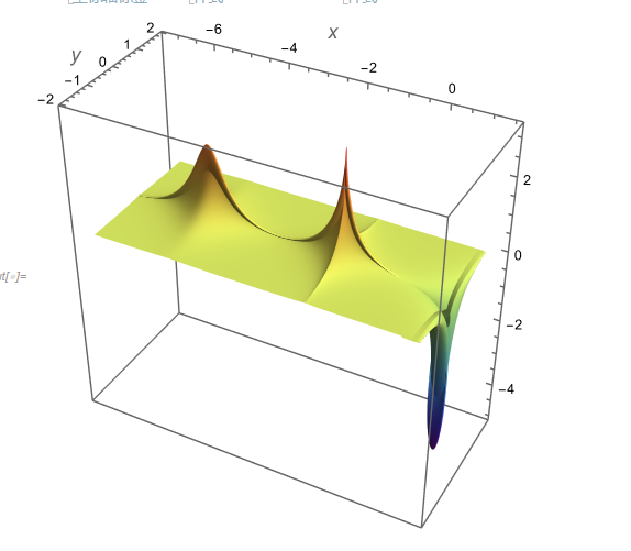
With[{t = -25},
With[{X = \[Xi] - 0.5 Tanh[\[Xi] - 0.3 t] - Tanh[\[Xi] - 0.1 t] -
1.5 Tanh[\[Xi] + 0.1 t], Y = \[Eta] - 1.15 Tanh[\[Eta]]},
ParametricPlot3D[{X, Y, func[\[Xi], \[Eta], t]}, {\[Xi],
4, -10}, {\[Eta], 3, -3}, PlotRange -> All, Mesh -> None,
PlotPoints -> 100, ColorFunction -> "Rainbow",
AxesLabel -> {Style[x, {15}], Style[y, {15}]}]]]
and it comes
Here, I would like to draw a 2D sectional plot for this 3D graphic at y=0, such as
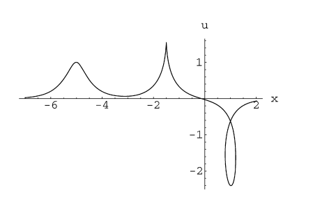
To achieve this goal, my code is
Y = 0;
With[{t = -25},
With[{X = \[Xi] - 0.5 Tanh[\[Xi] - 0.3 t] - Tanh[\[Xi] - 0.1 t] -
1.5 Tanh[\[Xi] + 0.1 t]},
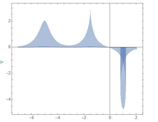
ParametricPlot[{X, func[\[Xi], \[Eta], t]}, {\[Xi],
5, -10}, {\[Eta], 3, -3}, PlotRange -> All, Mesh -> None,
PlotPoints -> 100, AxesLabel -> {Style[x, {15}], Style[y, {15}]}]]]
and it comes
How can I get the second picture(line sectional plot)?
cross-post: https://mathematica.stackexchange.com/questions/262040/how-to-draw-sectional-plot-for-a-3d-parameter-equation


