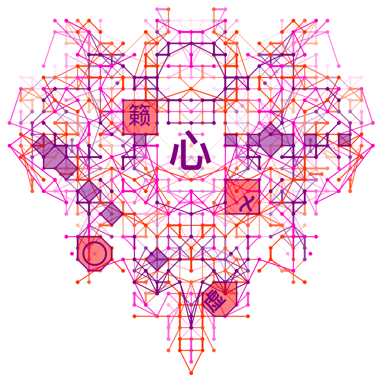
 Fig. 1. Music full heart, water tiger mountain mind.
Chinese New Year will continue until the Lantern Festival tomorrow, while in the western world, Feb. 14 is a special holiday for celebrating movements of the heart. The purpose of this memo is to show how a mysterious totalistic cellular automata, even if it isn't very well-defined, can still be used for purposes other than complicated math proofs. The goal is to find forms, such as above, and to put them into beating motion.
What is a totalistic Cellular Automaton? -------
A totalistic cellular automaton is a restricted type of cellular automaton, which calculates update values based on a total taken across a set of cells. First let's calculate codes of all totalistic elementary cellular automata:
TotalisticQ[code_, col_ : 2, rad_ : 1] := With[
 {totals = Total /@ Tuples[Range[0, col - 1], 2 rad + 1]},
  And @@ (SameQ @@ IntegerDigits[code, col, col^(2 rad + 1)][[
         Position[totals, #][[All, 1]]]] & /@ Union[totals])]

Flatten[Position[TotalisticQ[#] & /@ Range[0, 255], True] - 1]
Out[]={0, 1, 22, 23, 104, 105, 126, 127, 128, 129, 150, 151, 232, 233, 254, 255}
As an example, let's see what Rule 126 looks like starting from random initial conditions:
SeedRandom["PlotFun!"];
Image[CellularAutomaton[126,
  RandomInteger[1, 100], 100],
 ImageSize -> 400]
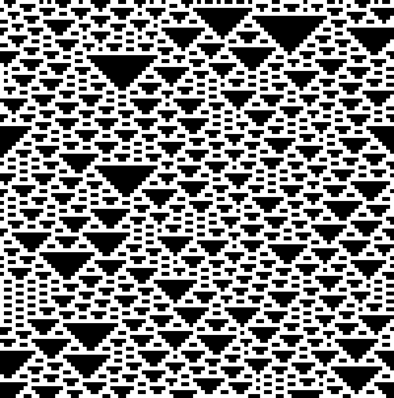
Notice that some of the triangles come to singular points, while others do not. This is an important, subtle detail if you are interested in studying Brownian motion--one of the topics from Einstein's miracle year. For now we're just having fun, not doing any serious science, but we may return to Brownian motion at a later time. It is also possible to plot the above using a slightly different call:
SeedRandom["PlotFun!"];
Image[CellularAutomaton[{6, {2, 1}},
  RandomInteger[1, 100], 100],
 ImageSize -> 400]
Out[]= (*Same as Above*)
When we compare alternative rules:
Column[MapThread[RulePlot[#1, ImageSize -> #2] &, {
   {CellularAutomaton[126], CellularAutomaton[{6, {2, 1}}]},
   {400, 200}}], Center]

We can see that the totalistic rule on the second line is four bits shorter, but still backwards compatible with the "elementary" definition on the first line. This is a nice feature of totalistic cellular automata, because small rule spaces are easier to search for interesting behavior.
Enigmatic Searching
Presently, we're concerned with finding a growth pattern that has a heart shape (♡) boundary. To get a heart shape to grow from a simple initial condition, we need a two dimensional cellular automaton, and guess a neighborhood shape function:
HeartNeighborhood = {{-1, 1}, {1, 1}, {-1, 0}, {1, 0}, {0, 0}, {0, -1}};
Graphics[Rectangle /@ HeartNeighborhood, ImageSize -> 50]

Okay, that looks like Ox Horns more than a heart, but let's just see what happens if we use this primitive to grow cellular automata. Next we introduce an admittedly confusing black-box code, something like this:
CAFirstArg[code_, transform_ : Identity] := {code, {4, 1},
 transform /@ HeartNeighborhood}
Don't ask me what this means or how it works exactly. This particular format for the first argument of the (too?) general CellularAutomaton function was shown to me in some other context, where rigor was not a high priority. Unfortunately, it's not well documented on the manual page, and RulePlot doesn't do anything either:
RulePlot[CellularAutomaton@CAFirstArg[1324123]]
Out[]:= (* nothing changes *)
[[Aside: In fact, now that I think about it, this might not even be a totalistic rule. We're not really trying to prove anything, so it doesn't exactly matter, for now. However, I am curious if anyone can explain what this code means in terms of an output equivalent, first principles implementation? If yes, perhaps we should file another bug report to add a missing value to RulePlot?]]
One thing we do know is that the number 4 indicates count of colors. The thinking behind this design choice is that four colors will give us enough degrees of freedom to create visually appealing patterns. If the rule is even totalistic (?), the number of valid codes is 4^19, where 4 is the number of colors, and 19 is the number of unique totals. Just as a quick, hackerish double check, we can try and see what happens if we call the C.A. evolution with too large a code:
CellularAutomaton[CAFirstArg[4^19], {{{1}}, 0}, 1]
Print:>CellularAutomaton::rsize: The specified rule number 274877906944
              is greater than the largest possible rule number (274877906943).
Thanks to nice error handling, we now know that codes must be integers between 0 and 4^19-1. This makes us a little more confident that it is a totalistic code (as we have been told by relevant authorities). Still a nagging doubt persists, as if "don't know" mind is never okay.
With so many possible codes, we can't do a simple brute force search. Fortunately for us, we don't immediately need Machine Learning or Genetic Algorithms. It is relatively easy to find heart shapes just searching randomly. Here is a basic, entry-level search function:
SearchCA[ntime_] := Quiet[With[{RandDat = DeleteCases[
      Rule[Show[#, ImageSize -> 200] &@Image[CellularAutomaton[
             CAFirstArg[#, Reverse], {{{1}}, 0}, {{{ntime}}}]/3],
         #] & /@ RandomInteger[{0, 4^19 - 1}, 100],  Rule[Image[{}], _]]},
   Select[RandDat, 10 < ImageDimensions[#[[1]]][[1]] < 2 ntime &]]]
The purpose of the selector at the end is to limit the search to smaller outputs, which seem to do a better job of exploring all possible boundary shapes. If the cutoff is changed to 5 or larger, many more results will be returned, mostly with a pentagonal shape reminiscent of baseball's home plate. Pentagonal cellular automata could be interesting in their own right, but for now lets see what we can find that look like hearts:
ResourceFunction["InteractiveListSelector"][SearchCA[25]]
Out[]=(* clickable search panel *)
It may take numerous searches to find exactly what you're looking for, but it's not too difficult to find heart-shaped candidates. When you do, just click the add button beneath interesting examples, then click copy and the codes go to the clipboard. Codes can then be pasted into curly brackets with ctrl-v. Here's the results of taking all from an example search:
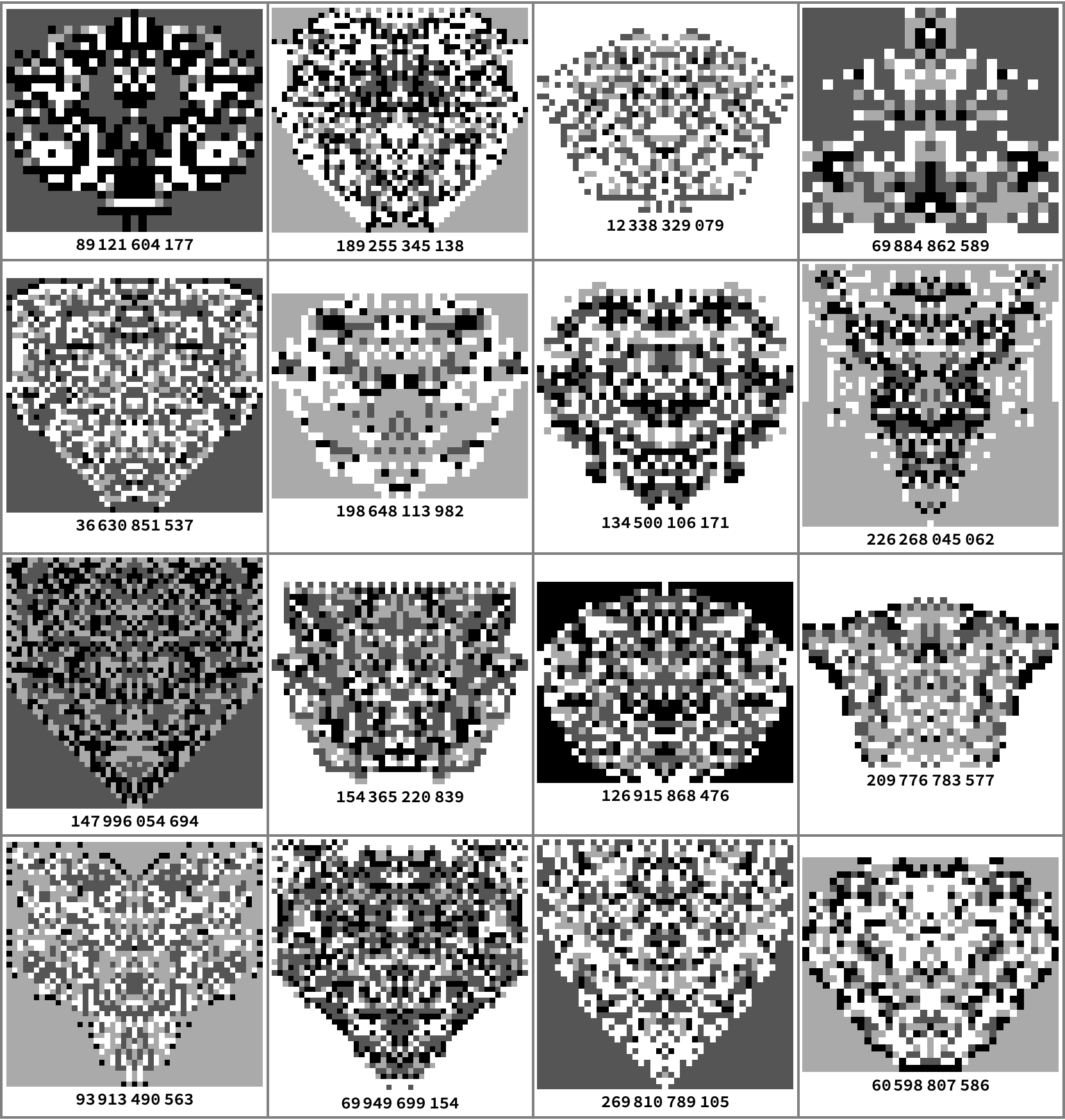
The case 134500106171 looks pretty well heart-shaped, as does the last element in the table 60598807586. Let's look at the evolution over time to see how the heart shape comes into existence as a time series:
Grid[Partition[  Image[# /. {0 -> {1, 1, 0}, 1 -> {1, 0, 0}, 2 -> {0, 1, 0},
       3 -> {0, 0, 1}},
     ImageSize -> 3 Reverse[Dimensions[#]]] & /@ CellularAutomaton[
    CAFirstArg[134500106171, Reverse], {{{1}}, 0}, {{0, 30}}], 5],
 Frame -> All, FrameStyle -> Directive[Lighter[Gray, 0.5], Thick]]
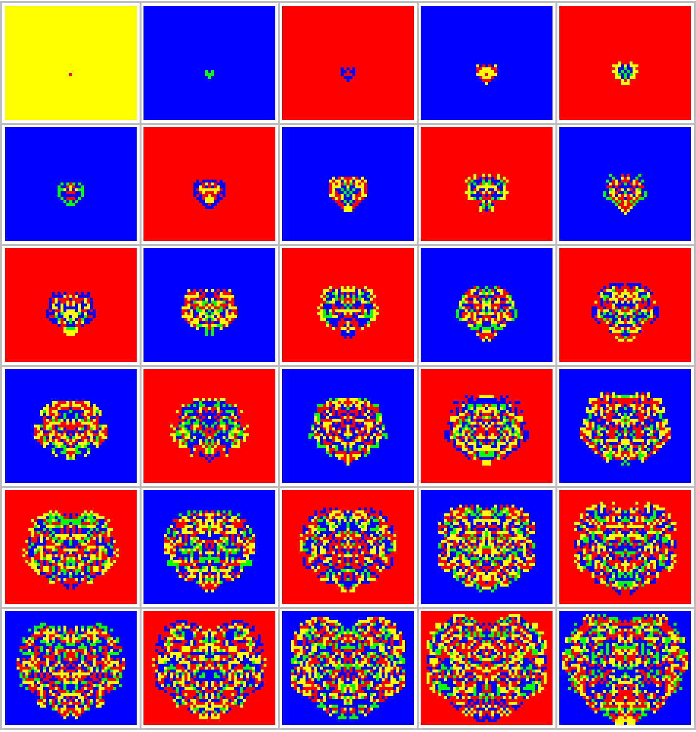
This is very nice already, and the tenth image, though small, also has quite a nice form. Even though we don't exactly know how this rule works, let's move on and possibly circle back to answer that question later. Instead of having an empty heart and a mind full of incomplete proofs, what we really need is a mind empty of doubt and a heart full of color (not to mention caring, compassion, etc.).
Building the Animation
After a little more searching I found another code, which produces really nice results: 113724623751. Let's see what this looks like for a few frames around t=25, and this time we are using a "sunset palette" with warm heart colors:
Grid[Partition[With[{glist = Image[# /. MapThread[Rule, {
           SortBy[Tally[Flatten[#]], -#[[2]] &][[All, 1]],
           {White, Blend[{Orange, Red}, .6],
            Blend[{Magenta, Red}, .25], Purple}
           }], ImageSize -> 4 Reverse[Dimensions[#]]] & /@
      CellularAutomaton[CAFirstArg[113724623751, Reverse],
 {{{1}}, 0}, {{22, 30 }}]}, glist], 3], Frame -> All,
 FrameStyle -> Directive[LightGray, Thick]]
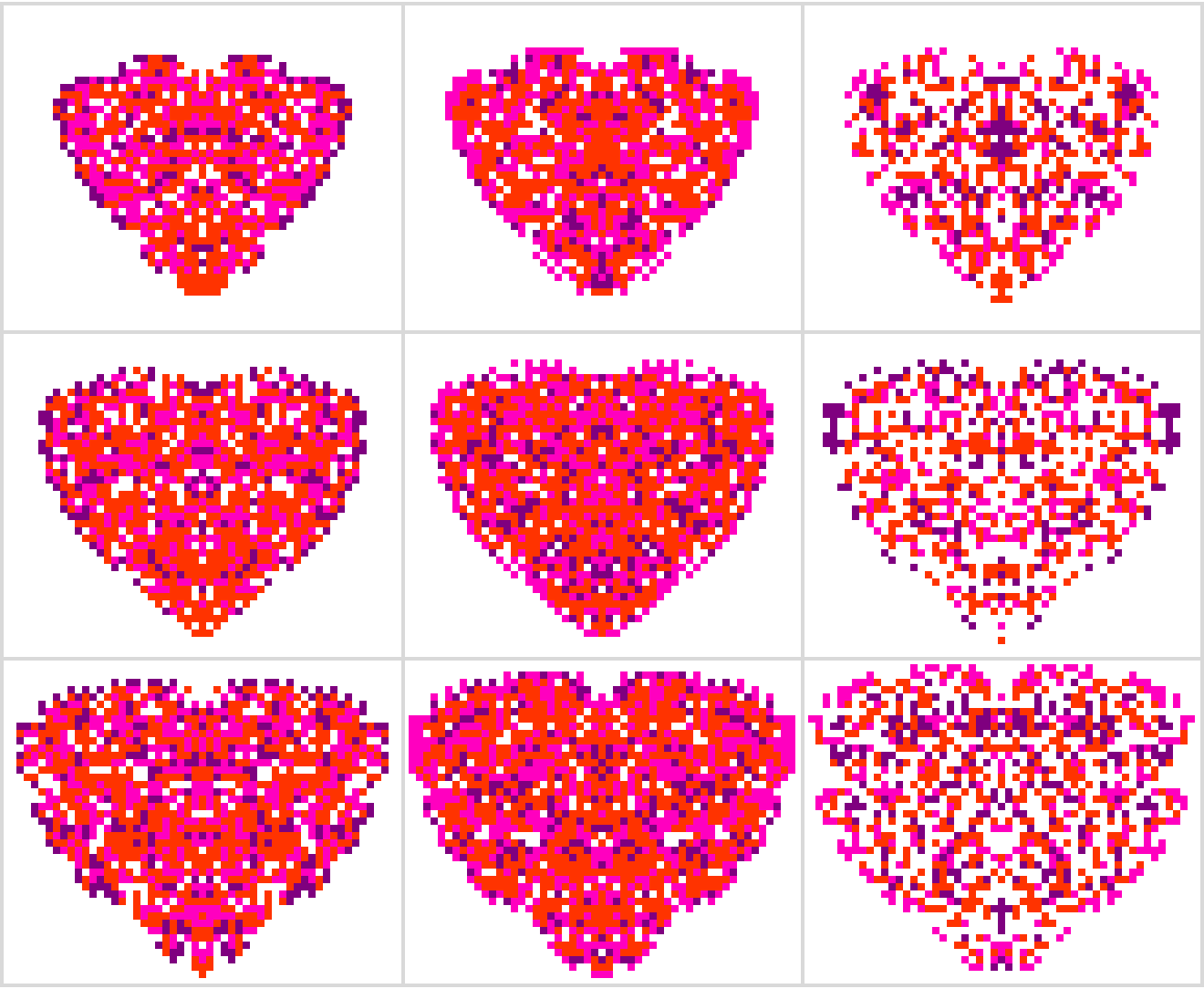
If you look more closely, the colors actually oscillate with period 3. We have hacked around this issue by sorting C.A. values according to their frequency statistics, thus attaining consistency between frames. With sorted colors, these outputs look pretty well like hearts. We can make them even more convincing with extra styling layers.
The basic idea is to separate colors, treat each vertex as a graph node, and draw in extra edges using the Nearest function. This is a design choice, which ultimately gives the images more texture, depth, and room to breathe. These next few functions are a bit of messy magic, but as they say, ends justify means.
GraphPattern[CA_, sort_, ColSets_, thick_ : 1/2, cut_ : Infinity] :=  Function[
   {NNEdges, NNNEdges}, Graphics[{
     Thickness[.005 thick],
     Transpose[{Reverse@{Purple, Blend[{Magenta, Red}, .25],
         Blend[{Orange, Red}, .6]},
       Reverse@Map[Line[{#[[1]], #[[2]]}] &, NNNEdges, {2}]}],
     Thickness[.01 thick],
     Transpose[{{Purple, Blend[{Magenta, Red}, .25],
        Blend[{Orange, Red}, .6]},
       Map[Line[{#[[1]], #[[2]]}] &, NNEdges, {2}]}],
     EdgeForm[None],
     Transpose[{{Purple, Blend[{Magenta, Red}, .25],
        Blend[{Orange, Red}, .6]},
       Map[Disk[#, 1/3 thick] &, ColSets, {2}]}]}]][
  Function[{oneCol}, Union[Flatten[
      Select[
        Edge[#, Nearest[Complement[oneCol, {#}], #]] & /@ oneCol,
        EuclideanDistance[#[[1]], #[[2, 1]]] == 1 &
        ] /. Edge[or_, ylist_] :> (Edge[or, #] & /@ ylist), 1]]] /@
   ColSets,
  Function[{oneCol}, Union[Flatten[
      Select[
        Function[{pt},
          Edge[pt, Nearest[Complement[oneCol, pt + # & /@ {
               {1, 0}, {0, 0}, {-1, 0}, {0, 1}, {0, -1}}], pt]]
          ] /@ oneCol, EuclideanDistance[#[[1]], #[[2, 1]]] <= cut &
        ] /. Edge[or_, ylist_] :> (Edge[or, #] & /@ ylist), 1]]] /@
   ColSets]

LayeredShieldGraph[CA_, sort_] := With[{BigColSets = Function[{oneCol},
        # + {1/2, 1/2} & /@
         Select[oneCol, Length[Intersection[oneCol,
              Function[{off}, # + off] /@ Tuples[{0, 1}, 2] ]] ==
            4 &]
        ][Position[CA, #]] & /@ sort},
  Show[GraphPattern[CA, sort, Complement[Position[CA, #],
       Flatten[Function[{or}, or + # & /@ Tuples[{1/2, -1/2}, 2]
          ] /@ Flatten[BigColSets, 1], 1]] & /@ sort],
   GraphPattern[CA, sort, BigColSets, 1/2, 3]]]

LayeredShieldGraph[code_, time_, sort_] :=
 With[{CA = CellularAutomaton[
     {code, {4,
       1}, {{0, 0}, {0, -1}, {-1, 0}, {1, 0}, {0, 1}, {0, 2}}
      }, {{{1}}, 0}, {{{time }}}]}, LayeredShieldGraph[CA, sort]]
Now the same data as above looks as follows:
Grid[data = Partition[With[{glist = LayeredShieldGraph[#,
         SortBy[Tally[Flatten[#]], #[[2]] &][[1 ;; 3, 1]]] & /@
       CellularAutomaton[
        CAFirstArg[113724623751, Times[#, {1, -1}] &],
        {{{1}}, 0}, {{22, 30 }}]}, glist], 3], Frame -> All,
 FrameStyle -> Directive[LightGray, Thick]]
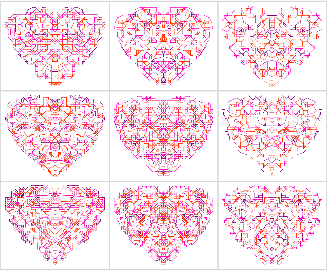
The view function does a little bit of extra work to introduce emptiness where numeric primitives have solid color. This works to our advantage, allowing us to enrich the pallette by stacking successive frames while fading to white:
LayeredHearts[code_, init_, final_, part_, fade_] := Show[
     Reverse[MapIndexed[#1 /. RGBColor[x_, y_, z_] :> Lighter[
          RGBColor[x, y, z], fade*( #2[[1]] - 1)] &, Reverse[#]]]] & /@
   Partition[With[
    {glist = LayeredShieldGraph[#, SortBy[Tally[Flatten[#]], #[[2]] &
           ][[1 ;; 3, 1]]] & /@
       CellularAutomaton[CAFirstArg[code, Times[#, {1, -1}] &],
        {{{1}}, 0}, {{init, final }}]}, glist], part, 1]

Grid[Partition[LayeredHearts @@ {113724623751, 22, 32, 3, 0.35}, 3],
 Frame -> All, FrameStyle -> Directive[LightGray, Thick],
 Background -> {None, None, {{3, 1} -> LightBlue}}]
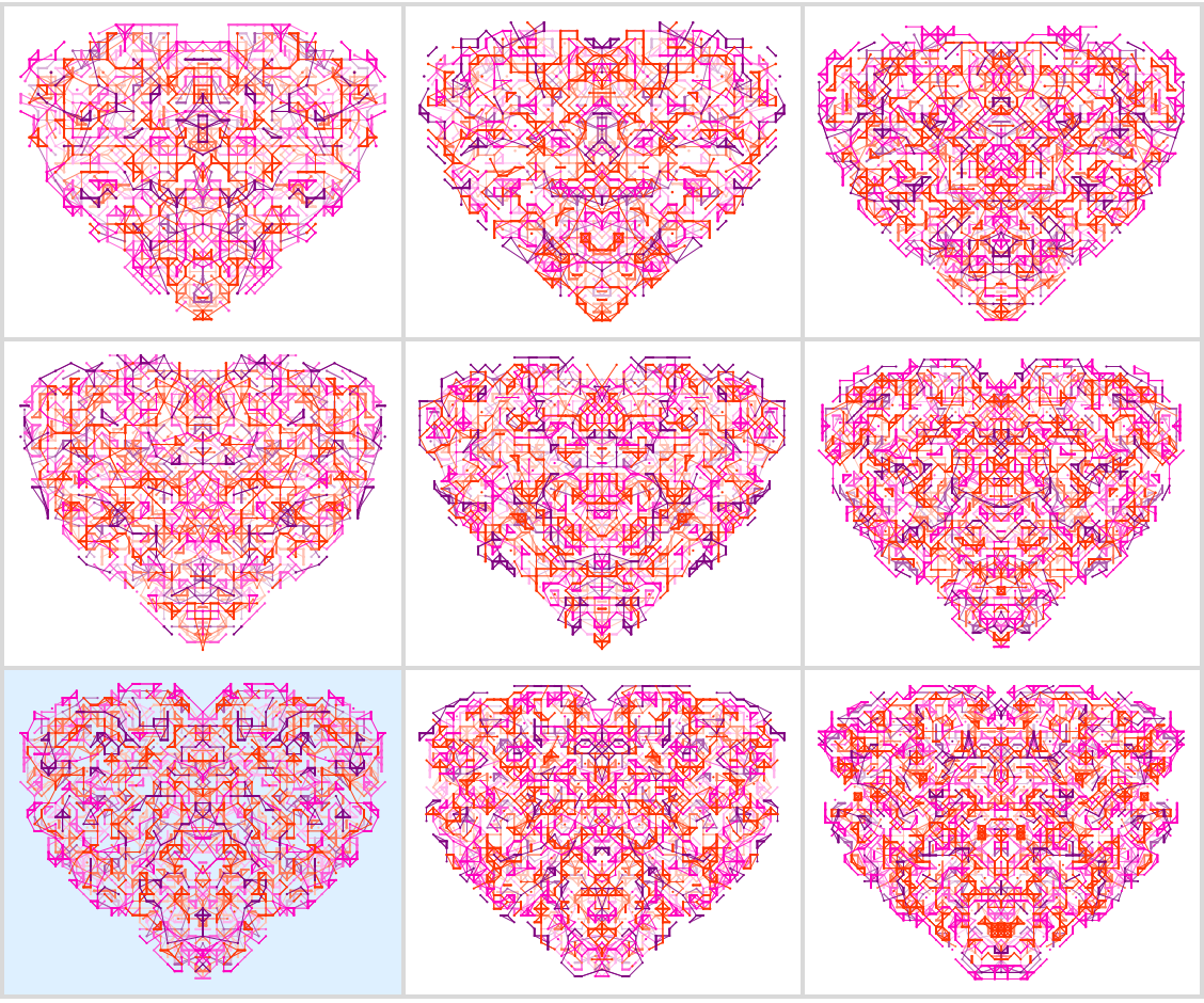
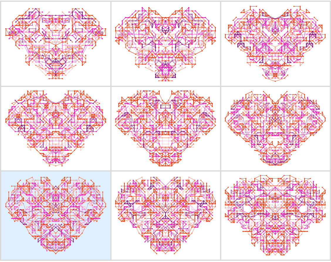
In the context of a time dynamic animation, the highlighted frame bottom left will be the beating hearts resting shape. The animation will cycle through surrounding frames according to a pulse shape that expands quickly, contracts for a slightly longer time interval, and ultimately returns to rest before repeating again:
PulseShape = {7, 7, 7, 8, 7, 6, 5, 4, 3, 2, 1, 2, 3, 4, 5, 6, 7, 8, 9,
    8, 7, 7, 7, 7, 7, 7, 7, 7, 7, 7};

AnimationData = Map[ Show[#, PlotRange -> {{-5, 63}, {-1, 51}}, ImageSize -> 620] &,
   Part[LayeredHearts @@ {113724623751, 22, 32, 3, 0.35},
    PulseShape]];

ListAnimate[AnimationData];
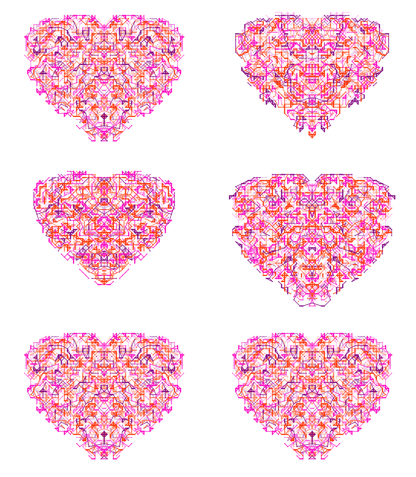
The feature I like about this particular plot is the purple Celtic cross occurring in the still frame, but I don't expect everyone to agree with me on preferences. If some other reader dislikes the purple cross, or more likely, desires some other boundary shape, that person can hopefully understand how to produce similar animations by changing only a few values: code, time window, stacking depth, and fade rate. Here is one more layout for example, or you can try to find your own:
Grid[Partition[LayeredHearts @@ {154655395227, 23, 35, 4, 0.25}, 3],
 Frame -> All,
 FrameStyle -> Directive[LightGray, Thick],
 Background -> {None, None, {{3, 1} -> LightBlue}}]
And the corresponding animation is:
AnimationData2 = Map[
   Show[#, PlotRange -> {{-5, 41}, {-3, 32}}, ImageSize -> 620] &,
   Part[LayeredHearts @@ {154655395227, 23, 35, 4, 0.25},
    PulseShape]];

ListAnimate[AnimationData2]
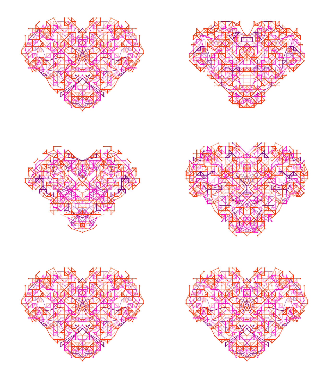
Happy Valentine's day... Don't forget the heart has it's own language entirely separate from what we think to say or to program in the computer!
Acknowledgements
The special form for C.A. first argument was known of by Stephen Wolfram, who told it to me at a meeting called by Danielle, thanks again!