Message Boards Message Boards

RandomSierpinskiMaze via Wolfram Function Repository

Posted 2 years ago

MODERATOR NOTE: this work was submitted to Computational Art Contest 2022. Check out the contest and other submissions here: https://wolfr.am/CompArt-22


fixed path counts
Fig. 1. Knight's walks, colored by path count summed over all possible starting points along the four exterior edges.

We are happy to announce the release of RandomSierpinskiMaze via Wolfram Function Repository. The documentation already gives an example how to chart a knight's walk through the maze, but for this post, let's take our explanation and plotting to the next fractal level!

The states adjacency graph is produced quite readily as:

RandomSierpinskiMaze = ResourceFunction["RandomSierpinskiMaze"];
SeedRandom["Compare"]; maze0 = RandomSierpinskiMaze[3, AdjacencyGraph];
Graph[#, VertexCoordinates -> (# -> # & /@ VertexList[#])] &@maze0

states adjacency

This graph assumes that the maze explorer moves by $\pm (0,1)$ or by $\pm (1,0)$. With knight's walks we allow and require that steps move by $(\pm1,\pm2)$ or $(\pm2,\pm1)$ for eight different choices of signs. (Knights are sometimes described as moving along a circle with radius $\sqrt{5}$.) The documentation also shows how to superimpose the states adjacency graph assuming the knight-walk transition function:

GraphUnion[maze0, kmaze0, 
 VertexCoordinates -> (# -> # & /@ VertexList[maze0]),
 EdgeStyle ->   Join[# -> Black & /@ EdgeList[maze0], # -> Orange & /@ 
    EdgeList[kmaze0]]] 

Knights graph

And if you look closely, you will see that knights can not achieve an ergodic limit when exploring possibilities of the maze. Their particular movement pattern locks them out of some corners, and makes it difficult to pass through narrow corridors.

Now we can find a difficult looking Knight's walk (in coordinate-free form):

KnightWalkGraph[graph0_] :=  With[{knightsMoves = 
    Flatten[  Outer[#1@{#2 2, #3 1} &, {Reverse, Identity}, {1, -1}, {1, -1}], 2]}, 
  Graph[Select[EdgeList[#], GraphDistance[graph0, #[[1]], #[[2]]] == 3 &]] &@
   Graph[ Union[ Sort /@ Select[
       Flatten[ Outer[UndirectedEdge[#1, #1 + #2] &, VertexList[maze0], 
         knightsMoves, 1]], MemberQ[VertexList[maze0], #[[2]]] &]]]]

kmaze0 =  With[{graph0 = KnightWalkGraph[maze0]}, 
  Graph[HighlightGraph[graph0, 
    PathGraph[FindShortestPath[graph0, {58, 13}, {83, 67}]]]]]

free form knights graph

Plenty of opportunities in there to get lost and take a wrong turn, but if you do, who knows what you will find! Even shortest paths between point A and point B can involve a fair amount of exploration:

With[{knightPath = FindShortestPath[kmaze0, {71, 1}, {83, 67}],
  arrayMaze = (SeedRandom["Compare"]; 
    RandomSierpinskiMaze[3][[1, 1]])  },
 animationData = ArrayPlot[ReplacePart[
       Reverse[arrayMaze], 
       Join[Reverse[# {1, -1} + {1, -1}] -> 2 & /@ Flatten[
            FindShortestPath[maze0, #1, #2][[2 ;; -2]] & @@@ 
             Partition[#, 2, 1], 1],
          Reverse[# {1, -1} + {1, -1}] -> 1 & /@ #] &@
        knightPath[[1 ;; #]]],
      PixelConstrained -> 8, ColorRules -> {
        4 -> LightGray, 5 -> White, 0 -> Black, 1 -> Orange, 
        2 -> LightOrange
        }] & /@ Range[Length[knightPath]];]

ListAnimate[animationData]

knights walk animation

This is just one particularly nice path. There are still many more paths to explore through this maze, and through other mazes generated from different seeds. And yes, if you have a metaverse strategy, mazes can be depicted in three dimensions (also thank the referees asking for extra revisions):

CarpetFractal[n_] :=  Nest[ArrayFlatten[{{#, #, #}, {#, 1, #}, {#, #, #}}] &, {{0, 0, 
    0}, {0, 1, 0}, {0, 0, 0}}, n]

ArrayMesh[Join[With[
    {mazebase = RandomSierpinskiMaze[3][[1, 1, 3 ;; -3, 3 ;; -3]
     ] /. {5 -> 0, 0 -> 1}}, Table[mazebase, {5}]], NestList[
    RotateRight[ Map[First[Sort@Commonest[Flatten[#][[{2, 4, 6, 8}]]]] &, 
       Partition[#, {3, 3}, {1, 1}, {1, 1}], {2}], {1, 1}] &, 
    CarpetFractal[3], 3^3 - 1]][[1 ;; -1 ;; 2]], ImageSize -> 500, 
 ViewVertical -> {1, 0, 0}, ViewPoint -> 2 {1.5, 1.5, 1}]

enter image description here

Have fun & use more colors as desired! For example, here's another interesting plot, where colors indicate that wall topology is different around top center:

another awesome plot

POSTED BY: Brad Klee
5 Replies

enter image description here -- you have earned Featured Contributor Badge enter image description here Your exceptional post has been selected for our editorial column Staff Picks http://wolfr.am/StaffPicks and Your Profile is now distinguished by a Featured Contributor Badge and is displayed on the Featured Contributor Board. Thank you!

POSTED BY: Moderation Team

Interesting. The mazes can be used into to texturize polyhedra:

img = Import["https://community.wolfram.com//c/portal/getImageAttachment?\filename=FindPartyMap.png&userId=234448"];
ResourceFunction["TexturizePolygons"][#, img, ImageSize -> Medium] & /@ {"Cube", "Octahedron", "SnubCube"}

enter image description here


img2 = Import["https://community.wolfram.com//c/portal/getImageAttachment?\filename=DifficultPath.gif&userId=234448"];
ResourceFunction["TexturizePolygons"][{#, "Net"}, img2, ImageSize -> Medium] & /@ {"Cube", "Octahedron"}

enter image description here


Similar effects can be achieved with RandomMondrian.

POSTED BY: Anton Antonov

Hi Anton, Thanks for the compliment, and your recent submission also looks very nice. I find that it sometimes helps meditation to have images such as these and to ponder or to simply appreciate their hidden and unknown dimensions.

One other thing to mention about the knight's walk graphs, which you may have noticed only by analysis, is that the red squares usually correspond to "safe spaces" in the following sense:

Imagine that you are just a pawn being pursued through the maze by an antagonistic knight. Most of the red squares are places where the knight could not attack you, because of its $(1,2)$ move pattern. After jumping around for a while, the knight would probably get bored and wander off to look for another (presumably innocent) target. Once the threat subsides, then you could go back to exploring the maze, probably with some part fear and anxiety what could be around the next corner.

This raises a question about game play: Let's assume instead you're playing the knight in battered armor, and that you are just trying to defend the maze from unwanted intruders. Are there any good strategies to capture pieces that are constrained to move to adjacent squares? Assume the knight knows the whole map, while pawns have limited, line-of-sight vision. Would there need to be more than one knight for efficient policing?

The other more creative question is about making mazes in three or more dimensions. Sierpinski carpet generalizes to Menger sponge. Anyone who gets the source code has a chance to figure out how to make 3D mazes, and perhaps the Sierpinski Octahedron could also be used as a template.

Alas, I don't think computational artwork is too high a priority, but it is a fun diversion that can possibly generate interesting and difficult test cases for potentially new and useful multicompuational algorithms. Hoping to make more progress along these lines soon...

POSTED BY: Brad Klee

While the chess knight can navigate through some narrow corridors, obviously the chess bishop can not. That is a less-than desirable theorem about the maze, because we also want a story problem about a bishop and actress who moves like a bishop. Have no fear, more WFR items are available to modify the game map, and now we can also see why the hue functions above are more than magic or art. First we get the extra resources:

RandomSierpinskiMaze = ResourceFunction["RandomSierpinskiMaze"];
SubmatrixReplace = ResourceFunction["SubmatrixReplace"]; 
ToDirectedAcyclicGraph = ResourceFunction["ToDirectedAcyclicGraph"];
DirectedAcyclicEvaluate = ResourceFunction["DirectedAcyclicEvaluate"];

And then we can almost immediately use SubmatrixReplace to widen the corridors:

SeedRandom["Compare"];
matrixData  = RandomSierpinskiMaze[3][[1, 1]][[2 ;; -2, 2 ;; -2]] /. {0 -> 1, 5 -> 0}

WidenCorridors = {{
     {0, _, n_, _, 0},
     {_, 1, 1, 1, _},
     {e_, 1, 1, 1, w_},
     {_, 1, 1, 1, _},
     {0, _, s_, _, 0}
     } :> {
     {0, 0, n, 0, 0},
     {0, 0, n, 0, 0},
     {e, e, 1, w, w},
     {0, 0, s, 0, 0},
     {0, 0, s, 0, 0}
     }};

bishopsMazeData = SubmatrixReplace[matrixData, WidenCorridors];

ArrayPlot[bishopsMazeData]

bishops maze

Alright, now we are hacking! The array data is good enough to generate new nearest-neighbor graphs:

nnpg = NearestNeighborGraph[Position[bishopsMazeData, 0]];

nnbpg = NearestNeighborGraph[Position[bishopsMazeData, 0],
   {All, Sqrt[2]}, GraphLayout -> "SpringElectricalEmbedding"];

nnbg = Graph[Complement[EdgeList[nnbpg], EdgeList[nnpg]],
  VertexCoordinates -> (# -> # & /@ VertexList[nnpg])]

bishop graph

And if you look closely, there are actually $2$ components to the graph, sometimes the black and white of a checkerboard, but also separate domains for the bishop and the actress.

Now, before we move on to the drama, let's get a better sense of the maze's particular topology. And even before even doing this let's calibrate our measurement instrument on a simple grid:

calibrationGraph = GraphUnion[
   NearestNeighborGraph[
    Position[Array[Mod[#1 + #2, 2] &, {30, 30}], 1]],
   NearestNeighborGraph[
    Position[Array[Mod[#1 + #2, 2] &, {30, 30}], 0]]
   ];

WalkColorArray[graph_, dims_] := Module[
  {initConditions = Cases[VertexList[graph],
     {1, _} | {_, 1} | {dims[[1]], _} | {_, dims[[2]]}],
    matrixData,  summedData, counts, countsRep},
  matrixData = ReplacePart[
      Array[0 &, dims],
      DirectedAcyclicEvaluate[#,
        {{_, _} -> 1}]["VertexWeights"]
      ] &@ToDirectedAcyclicGraph[graph, initConditions];
  summedData = matrixData;
  summedData = ReplacePart[summedData,
    # -> -1 & /@ Select[VertexList@graph,
      Part[summedData, Sequence @@ #] == 0 &]];
  counts = DeleteCases[Union[Flatten[summedData]], 0 | -1];
  countsRep = MapIndexed[#1 -> #2[[1]] &, counts];
  ArrayPlot[summedData,
   ColorRules -> Join[# -> Lighter[Hue[
          (# /. countsRep)/Length[counts]/1.1
          ], .5] & /@ counts, {0 -> Black, -1 -> Red}],
   Frame -> None, PixelConstrained -> 8]]

WalkColorArray[calibrationGraph, {30, 30}]

calibration

The best way to understand the measurement is to actually read the source code, but the calibration image is also instructive. Colors measure counts of shortest paths starting from any point on the edge. As time goes on, paths branch and merge, causing path count to increase toward the center of the array. Effectively, this path count function also acts almost like a distance function. It's not the best measurement, but at least it doesn't depend on a particular entry point.

And for the maze we get:

WalkColorArray[nnbg, {83, 83}]  

enter image description here

This is not much different from the graph we calculated previously for knights, but notice that the "center" has split with a large part shifted to south west. Or as disconnected graph components:

enter image description here

Let's look a little more closely at the "center", which is so defined because the greatest number of shortest paths lead there:

initConditions = Cases[VertexList[nnbg],
   {1, _} | {_, 1} | {83, _} | {_, 83}];

directedBg = ToDirectedAcyclicGraph[nnbg, initConditions];

inits = Cases[VertexInComponent[directedBg,
      {#, 62}], {1, _} | {_, 1} | {83, _} | {_, 83}] & /@ {22, 23};

inComp = VertexInComponent[directedBg, {#, 62}] & /@ {22, 23};

Graph[nnbg,  VertexCoordinates -> (# -> (# {1, -1}) & /@ VertexList[nnbg]),
 VertexStyle ->   Join[# -> Magenta & /@ inComp[[1]], # -> Orange & /@ inComp[[2]],
   {{22, 62} -> Red, {23, 62} -> Red}]] 

center paths

Well, admittedly this is somewhat disappointing. We find that the ensemble of shortest paths all originate from one simply connected region on the west boundary. This is a consequence of how we have chosen an overly-simple transformation from the adjacency graph into a directed acyclic graph. For dramatic purposes, we would rather have magenta and orange paths starting from widely separate entry points.

We can always make more complicated graph transformations (and don't worry, we will), but for now our first simple idea has other acceptable possibilities. The secluded blue and magenta checkerboard near north center looks to be a likely place for a meeting of the bishop and the actress, and yes it is:

meeting graph

There are multiple entry points that allow the orange and magenta players to access the meeting on a shortest path, so we just choose two, and animate the cutscene:

meeting animation

This is almost exactly what we want for possible game play, but is it realistic that the bishop and the actress know the maze and this particular location so well? How about instead, if the chosen graph transformations allowed them to get lost? Would the meeting still happen? And should there be more characters in on the board? Stay tuned...

POSTED BY: Brad Klee

MODERATOR NOTE: a submission to computations art contest, see more: https://wolfr.am/CompArt-22


enter image description here

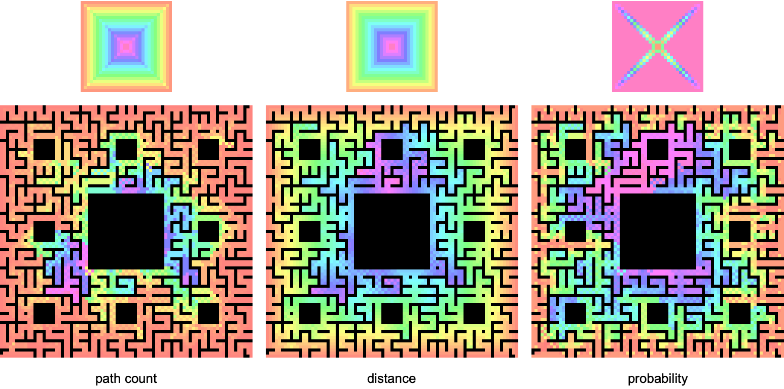
Actually there is no obvious definition for the center of a maze, so we might as well try a few more calculations using DirectedAcyclicEvaluate. The graphs above are made with three different choices of vertex function:

nnbgDAG = ToDirectedAcyclicGraph[nnbg, Cases[VertexList[nnbg],
    {1, _} | {_, 1} | {83, _} | {_, 83}]];

pathCount = Function[{values, edgeWeights, edges},Total[values] ];

distance = Function[{values, edgeWeights, edges},  values[[1]] + 1 ];

probability = Function[{values, edgeWeights, edges},
   Total[Times[values,1/VertexOutDegree[nnbgDAG, 
      #] & /@ edges[[All, 1]]  ] ] ]; 

It would be a little more sophisticated to calculate probabilities using edge weights, but presently the source code is missing an important optimization using Association (see end note below). It's interesting to compare these functions, and such analysis can possibly help us find our way past the center of the maze and to escape, whatever that actually means.

Assuming a maze explorer can start anywhere on the boundary and moves with constant velocity, minimum distance from the wall to any interior point is proportional to minimal time. Thus distance acts as a time axis, which increases toward magenta. The probability function is correlated to the distance / time function because, as time goes on, maze explorers run out of space to explore. More definitely said, the probability function equally splits values when through-putting along directed edges, so a partial probability amplitude is conserved from time $t$ to $t+1$ only if its location in the maze graph has at least one out component as a next move. As this is not the case for the entire graph, we observe the probability amplitude falling off exponentially with distance / time:

leveledVertices = SortBy[GatherBy[
     DirectedAcyclicEvaluate[nnbgDAG,
       {{_, _} -> 1}, distance]["VertexWeights"],
     #[[2]] &], #[[1, 2]] &][[All, All, 1]];

probs = Total /@ (leveledVertices /. DirectedAcyclicEvaluate[ nnbgDAG,
      {{_, _} -> 1}, prob]["VertexWeights"]);

ListPlot[probs/276, PlotRange -> All, 
 AxesLabel -> {"distance/time", "probability"}]

maze tunneling

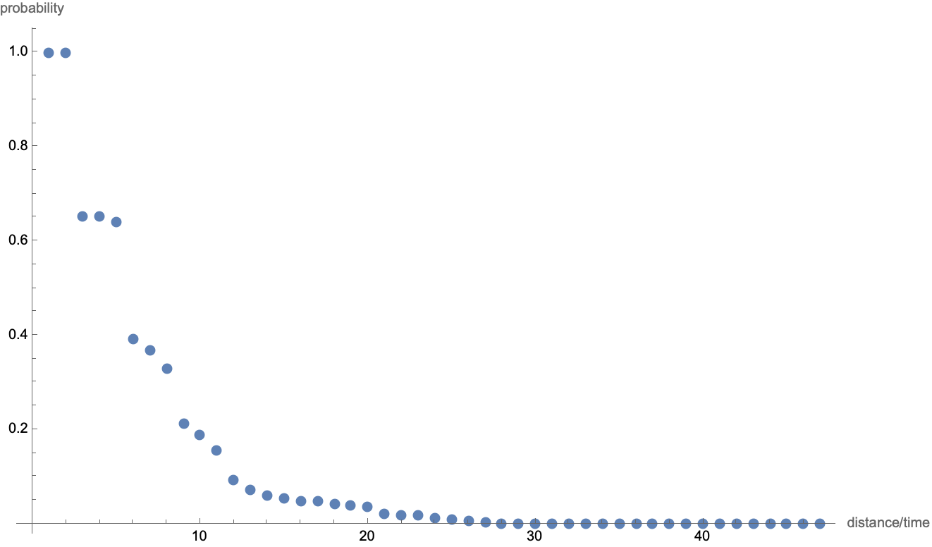
This plot somewhat reminds us of quantum mechanical tunneling, but I'll refrain from speculating about possible future physics directions. The graph functions don't account for Schroedinger phases (yet), so there's really no need to mention Quantum.

We previously mentioned a limitation to the metrics above is that, for any chosen starting point, the underlying directed acyclic graph does not reach out to every other location of the maze. In practice, this limits the drama from what it could possibly be when allowing characters to take paths across the entire maze.

One way to correct this deficit is to use only one starting location when calculating the shortest path map of the maze. If we then make shortest path graphs for every possible initial condition, we can sum over all initial conditions to obtain a new set of more detailed measurements of the maze. Now for a little more code:

compGraphs = WeaklyConnectedGraphComponents[nnbg];
initConditions = Cases[VertexList[#],
     {1, _} | {_, 1} | {83, _} | {_, 83}] & /@ compGraphs;

dags1 = ToDirectedAcyclicGraph[compGraphs[[1]], {# },
     VertexCoordinates -> Automatic
     ] & /@ initConditions[[1]];

dags2 = ToDirectedAcyclicGraph[compGraphs[[2]], {# },
     VertexCoordinates -> Automatic
     ] & /@ initConditions[[2]];

matrixPathData = Function[{graph},
    ReplacePart[Array[0 &, {83, 83}],
     DirectedAcyclicEvaluate[graph,
       {{_, _} -> 1}]["VertexWeights"]]] /@ dags;

matrixProbData = Function[{graph},
    ReplacePart[Array[0 &, {83, 83}],
     DirectedAcyclicEvaluate[graph,
       {{_, _} -> 1},
       Function[{values, edgeWeights, edges},
        Total[Times[values,
          1/VertexOutDegree[graph, #] & /@ edges[[All, 1]] ] ] ]
       ]["VertexWeights"]]] /@ dags;

matrixDistData = Function[{graph},
    ReplacePart[Array[0 &, {83, 83}],
     DirectedAcyclicEvaluate[graph,
       {{_, _} -> 1},
       Function[{values, edgeWeights, edges},
        values[[1]] + 1 ]
       ]["VertexWeights"]]] /@ dags;

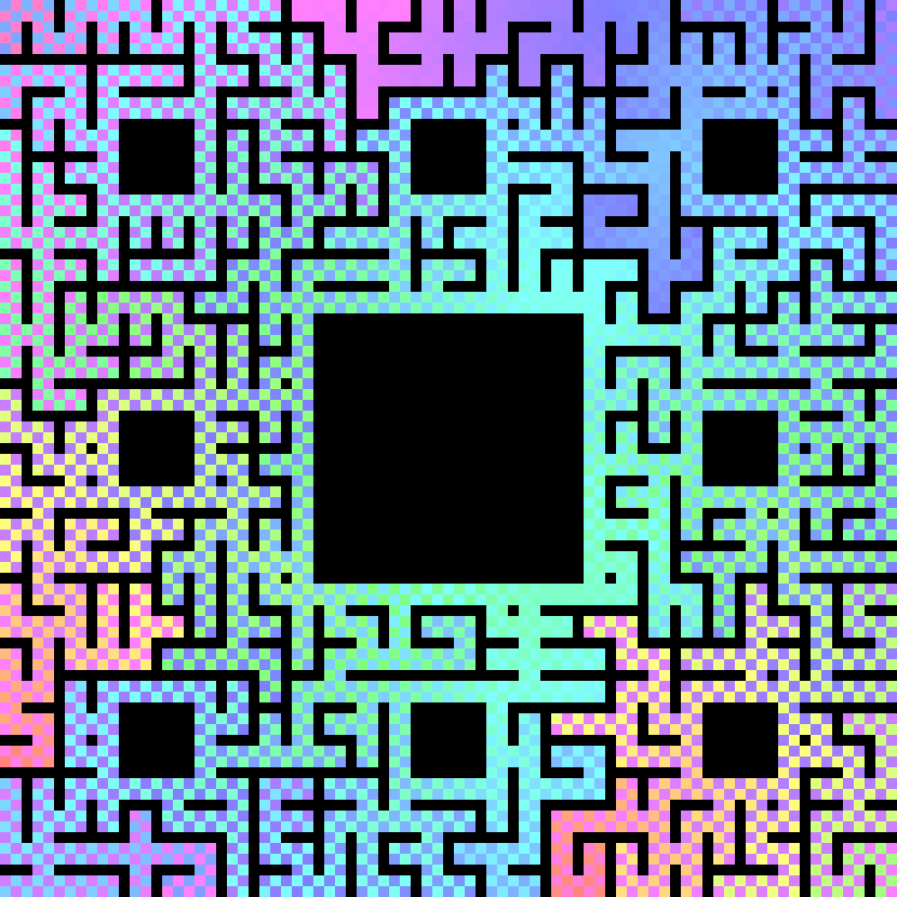
All told it takes about 5-10 minutes to do a similar calculation over 250+ initial conditions, and then we can plot the revised metrics:

HueScaleArrayPlot[summedData_] := With[
  {countsRep = MapIndexed[#1 -> #2[[1]] &,
     DeleteCases[Union[Flatten[summedData]], 0 | -1]]},
  ArrayPlot[Transpose@summedData,
   ColorRules -> Join[# -> Lighter[Hue[
          (# /. countsRep)/Length[countsRep[[All, 1]]]/1.1
          ], .5] & /@ countsRep[[All, 1]], {0 -> Black, -1 -> Red}],
   Frame -> None, PixelConstrained -> 3]]

HueScaleArrayPlot[Total[#]] & /@ {matrixPathData, matrixDistData, 
  matrixProbData}

measurement 2

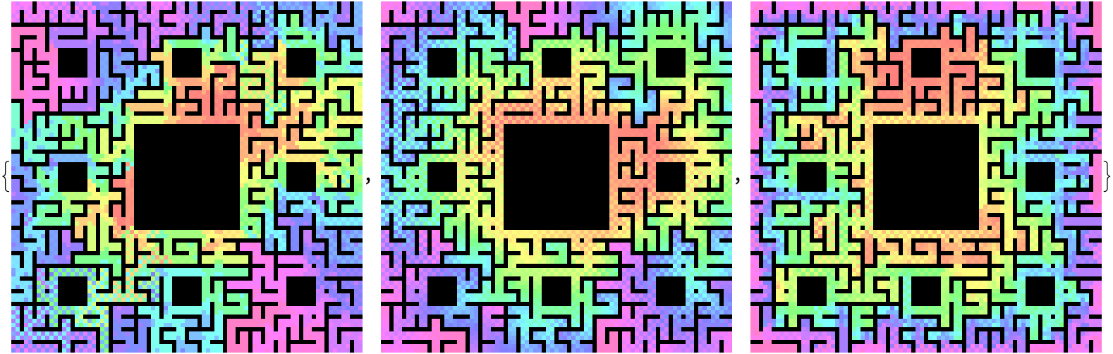
Higher precision path count and distance measurements are more sensitive to the difficult of accessing certain exterior sections of the maze. The probability metric changes less significantly, continuing to highlight north center as the most difficult region to reach.

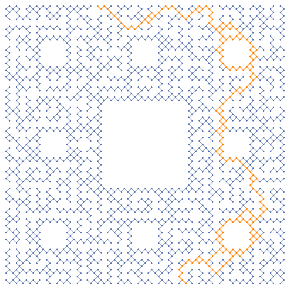
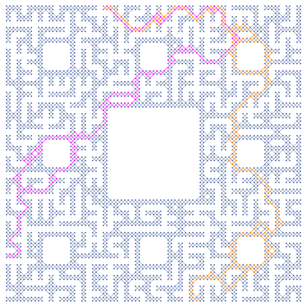
Let's assume for the next play, the bishop and the actress are going to enter the maze from different directions, and attempt to synchronize their movements so as to end up leaving the maze together on a distinct third direction. For one path, It is possible to enter South East and exit North center, choosing both endpoints in bottlenecked subspaces. We can plot the multiway subgraph as follows:

VertexKeep[graph_, vertices_, OptionsPattern[Graph]
  ] := VertexDelete[graph,
  Complement[VertexList[graph], vertices],
  Sequence @@ (#[[1]] -> OptionValue[#[[1]]] & /@ Options[Graph])]

Graph[HighlightGraph[compGraphs[[1]],
  Style[VertexKeep[compGraphs[[1]],
    VertexInComponent[dags1[[139]], {28, 1}, Infinity]],
   Orange, Thick]], VertexCoordinates -> (
   # -> Times[#, {1, -1}
       ] & /@ VertexList[dags1[[139]]]), ImageSize -> 500]

path 1

Now by fixing one component of matrix distance data and scanning over components on the second sublattice, we can look through pair correlations to try and find a synchronous partner function:

unsorted = # - Mean[initConditions[[2]]] & /@ initConditions[[2]];
sorted = SortBy[unsorted, N[(ArcTan @@ # + Pi)] &];
inds = Flatten[Position[unsorted, #] & /@ sorted];

correlationData = 
  HueScaleArrayPlot[matrixDistData[[139]] + matrixDistData[[140 + #]]
     ] & /@ Join[Range[139][[inds]], Table[272 - 140, {50}]];
ListAnimate[%]

pair correlations

In this image player 1's starting point is fixed while player 2's starting point rotates clockwise around the boundary. In the end, we find one particularly nice and synchronous convergence of separate paths:

Image[HueScaleArrayPlot[
  matrixDistData[[139]] + matrixDistData[[272]]
], ImageSize -> 6*83]

two paths

And the $(A_1,A_2) \rightarrow B$ multiway subgraph function looks as follows:

paths graphs

It looks like a pretty good plan, but not if king so-and-so (or perhaps one of the saintly seven) happens to hear about it. Whatever pre-existing powers may not see it in their interest that the Bishop and the Actress should meet in the maze and end up leaving together. The scene is much more dramatic if the players have a chance of being intercepted by knights patrolling around maze cycles:

no new meeting

Of course, it's always possible to choose another random seed, and then the meet-and-escape can happen despite the menacing presence of the blue knights:

meeting does happen

These plots prove a concept, but leave more to desire. Shouldn't the players have more of an ability to avoid knights? And shouldn't the knights make more of an effort to give chase? Yes, of course, but please don't discredit incremental progress on account of a future that doesn't yet exist.

End Note

Pay attention to this timing test, now not to use replace rules:

rules = # -> # & /@ Range[1000];
rulesf = Association[rules];
t1 = RepeatedTiming[rulesf[RandomInteger[1000]]];
t2 = RepeatedTiming[RandomInteger[1000] /. rules];
t2[[1]]/t1[[1]]

Out[] > 75
POSTED BY: Brad Klee
Reply to this discussion
Community posts can be styled and formatted using the Markdown syntax.
Reply Preview
Attachments
Remove
or Discard

Group Abstract Group Abstract