I thought I would share the following rather simple experiment. It is based on a Geiger counter which interacts via the serial port with Mathematica. It can be used to measure ambient levels of radioactivity and to test different radioactive sources at home. As an additional benefit it generates "perfect/physical" random numbers (as opposed to pseudorandom numbers), some of which I attach to this post.
The setup is rather simple, unfortunately one of the parts is a bit expensive. I use
1)
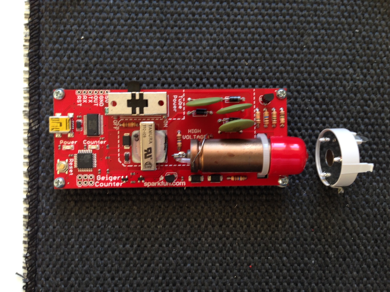
Sparkfun's Geiger Counter SEN-11345. (about 150 $ and similar in £)
2) A USB 2.0 A/Mini-B cable.
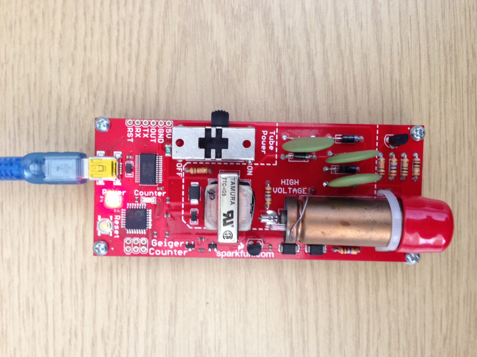
The Geiger tube is on the bottem right on the photo. The parts inside the dashed line are under high voltage when the thing is switched on; avoid touching any of these parts. The Geiger counter has an onboard AMTEL chip (like Arduino) so it communicate easily via the serial port. You might have to install the appropriate VCP driver
from this website.
Once the driver is installed you connect the Geiger counter to the USB port of the computer. On the software side you need to install the
SerialIO package. Step by step instructions for the installation can be found on
this website.
The Sparkfun Geiger counter sends a sequence of 0 and 1 to the serial port, which indicate whether the previous interval is longer or shorter than the current interval between counts. Each number corresponds to one event - the counter measures alpha, beta and gamma radiation; the latter only if the red protective cap is removed. The sequence of zeros and ones can be used as a set of independent random numbers. For most simulations the pseudorandom numbers that computers (and Mathematica) generate, but for some other applications such as encryption physical random numbers are preferable. The code below will produce that string of random digits, but it will also record the times of the measured decay events. The code is for Mac OSX but can easily be adapted for other operating systems.
(*Clear everything*)
ClearAll["Global`*"]
(*Load SerialIO*)
<< SerialIO`
(*Connect to the Geiger counter*)
myGeigerCounter =
SerialOpen[Quiet[FileNames["tty.usb*", {"/dev"}, Infinity]][[1]]];
SerialSetOptions[myGeigerCounter, "BaudRate" -> 9600];
While[SerialReadyQ[myGeigerCounter] == False, Pause[0.1]];
(*Measure*)
s = {}; tZero = AbsoluteTime[]; SerialRead[myGeigerCounter];
Dynamic[
Refresh[
AppendTo[s, {SerialRead[myGeigerCounter], AbsoluteTime[] - tZero}];,
UpdateInterval -> 0.002],
SynchronousUpdating -> False]
That is basically the entire code for reading the data. The critical point is the UpdateInterval. If the computer is busy, it might measure too slowly and measure a sequence of 0s and 1s instead of a single digit, so it is important to have few background processes running. The UpdateInterval of 0.002 has shown to be sufficiently high for my experiments; Sparkfun's detector can measure up to 100 Hz. Also, if there is no event for 10 seconds the program will read " " and record the time, i.e. last event plus 10 seconds. Therefore we need to clean up the data after the measurement is finished (simply abort the evaluation), see below. If you want to plot the measurements dynamically you can use:
Dynamic[sc = DeleteCases[s, {"", ___}];
ListPlot[sc[[2 ;;, 2]] - sc[[1 ;; -2, 2]],
PlotRange -> {All, {0, Max[sc[2 ;;, 2]] - sc[[1 ;; -2, 2]]}},
ImageSize -> Large]]
This gives the following animation, where every couple of seconds a new point is added.
If you are interested in an estimate of the "counts per minute" this command will do the trick:
Dynamic[10/(sc[[-1, 2]] - sc[[-10, 2]])*60. // N]
So by now we have a working Geiger counter and we can visualise the results.
To test the counter I ran a measurement of the background radiation for a couple of hours. I import the data:
tstest = Import["~/Desktop/Geigerdata_overnight.csv"];
Then clean it up
tsBackground = DeleteCases[# & /@ tstest, {"", ___}] // ToExpression
and plot a diagram of the time between two consecutive events
ListPlot[tsBackground[[2 ;; -1, 2]] - tsBackground[[1 ;; -2, 2]],
PlotRange -> All, AxesLabel -> {"Decay Incidence", "Waiting Time"},
ImageSize -> Large]
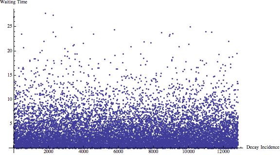
There are sligthly more than 12000 events in this time series.
To compare that to some radioactive object I dismantled a smoke detector and extracted the radioactive Americanum 241 container. The sourse emits alpha and gamma particles and is supposed to have a rate of about 33000 Bq, i.e. decays per second. (It says 0.9uCi on the detector. Wolfram Alpha knows that that is 33300 Bq.)
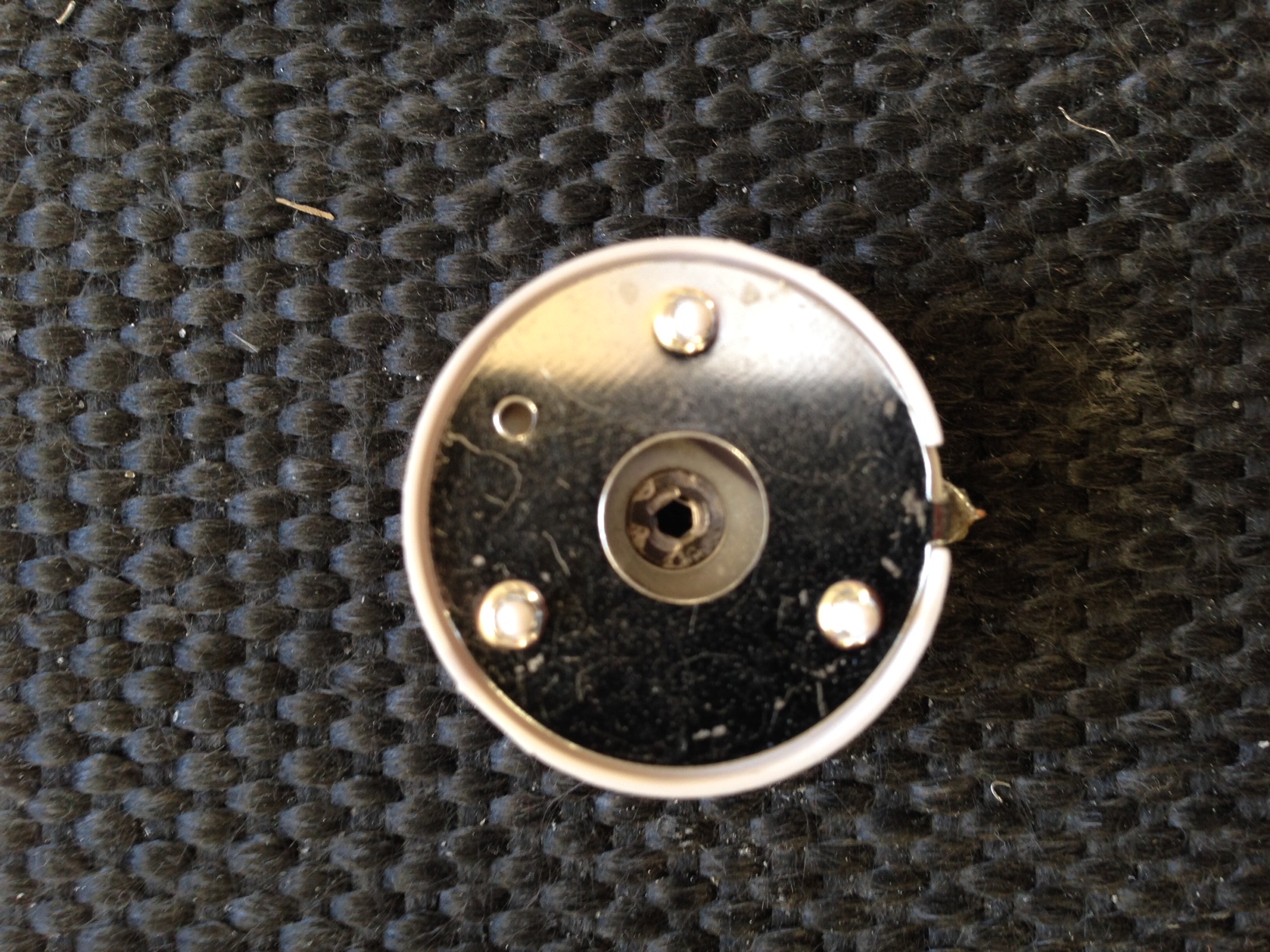
I position the Americanum at about 3 cm from the tip of the Geiger counter.
I then measure the counts over a couple of hours and obtain:
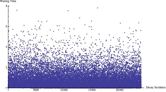
This time there are more then 20000 events recorded. Note that the waiting times are much shorter than in the background case. We can now compare the histograms of the waiting time between two consecutive events:
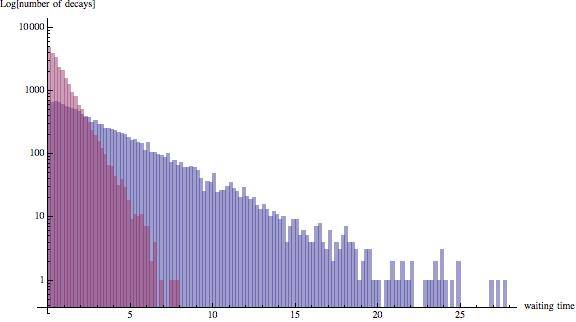
The total number of events are not the same, but it is obvious that the waiting times are much shorter for the Americanum element than for the background (blue).
The waiting time distribution is expected to be exponentially distributed, so we can fit
distBackground =
EstimatedDistribution[
tsBackground[[2 ;; -1, 2]] - tsBackground[[1 ;; -2, 2]],
ExponentialDistribution[\[Mu]]]
which gives
ExponentialDistribution[0.302391]
and
distAmericanum =
EstimatedDistribution[
tsAmericanum[[2 ;; -1, 2]] - tsAmericanum[[1 ;; -2, 2]],
ExponentialDistribution[\[Mu]]]
which gives
ExponentialDistribution[1.15882]
The mean waiting time for the background is
Mean[distBackground]
(*3.30698*)
and for the Americanum element
Mean[distAmericanum]
(*0.862946*)
Here is another representation
Show[{ListLinePlot[
Transpose[{HistogramList[
tsBackground[[2 ;; -1, 2]] - tsBackground[[1 ;; -2, 2]]][[
1]][[;; -2]],
HistogramList[
tsBackground[[2 ;; -1, 2]] - tsBackground[[1 ;; -2, 2]]][[
2]] // Log // N}], Mesh -> All,
AxesLabel -> {"waiting time", "Log number"}, ImageSize -> Large],
ListLinePlot[
Transpose[{HistogramList[
tsAmericanum[[2 ;; -1, 2]] - tsAmericanum[[1 ;; -2, 2]]][[
1]][[;; -2]],
HistogramList[
tsAmericanum[[2 ;; -1, 2]] - tsAmericanum[[1 ;; -2, 2]]][[
2]] // Log // N}], PlotStyle -> Red, Mesh -> All]}]
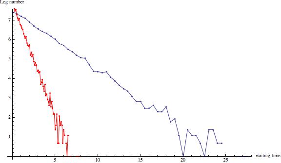
Wolfram Alpha knows a lot of useful stuff about Americanum 241, try:
== AM 241
One little issue with the measurement is that the Americanum element is supposed to have 33000 Bq, i.e. decays per second. Our measurement, corrected for background radiation, shows that there is more or less one additional decay per second. When the measurement was conducted, the red cap at the tip of the Geiger counter was not removed; this filters out the alpha radiation. I read somewhere that only less than 10% of the events come from gamma radiation, even though that seems incorrect given the information on
wikipedia. Also the detector was at a distance of about 3 cm from the element. Its opening is about 1cm^2. That might account for another factor of 100, but we would still be much below the at least 33 events per second. I have not really looked into this or done any calculations, but it might be nice to find the missing events.
This does not seem to be a problem with the 0.002 Updateinterval, as visual inspection of the time series shows that there are nearly no incidence of two bits being read at the same time from the serial port. The Geiger conter can measure up to 100Hz. The counts per minute of the background radiation are about 20 which is reasonable. (The measurement was made in Aberdeen (UK) where many houses are made from Granite which is slightly radioactive. Inside the hoses Radon is produced which can sometimes yield very high levels of radiation. This particular measurement was not taken in a Granite house.)
If anyone cares about good random numbers, they can use
tsAmericanum[[All, 1]]
To extract a string of ones ans zeros, which are "real" random numbers. I attach a file with the sequence of ones and zeros I got from the Americanum experiment. You can also use that to analyse how many times our update interval was too slow so that two digits were transmitted at once. The file can be read with:
data = Import["~/Desktop/RandomAmericanum.csv"] // Flatten
A simple Tally shows that
Tally[data]
(*{{0, 11779}, {1, 11979}, {11, 65}, {10, 1}}*)
Only 66 cases out of about 22000 were double digits.
Much about the code can/should be improved. Using an intermediate Arduino might improve the measurements slightly.
M.
PS: Note that there might be regulations in your country regarding the Americanum element of the smoke detector, e.g. how to dispose of them. Also Sparkfun does not deliver the Geiger Counter to all countries.
 Attachments: