It is good to have lots of examples...
SeedRandom[123123];
g1 = Graph[
WeaklyConnectedGraphComponents[
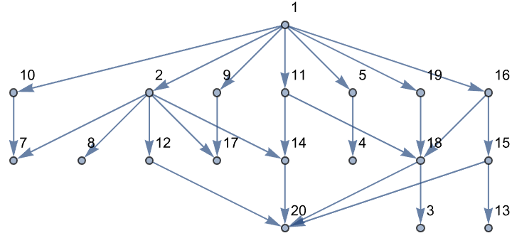
ResourceFunction["ToDirectedAcyclicGraph"][RandomGraph[{20, 40}],
1]][[1]], VertexCoordinates -> Automatic, VertexLabels -> "Name",
GraphLayout -> Automatic]
Mathematica has functions like BacktrackSearch for resource functions, yay!
ResourceFunction["BacktrackSearch"][{{1}, VertexList[g1],
  VertexList[g1], VertexList[g1]},
 MemberQ[EdgeList[g1], DirectedEdge @@ #[[-2 ;; -1]]] &, True &, All]
knightMoves = {{-2, -1}, {-2, 1}, {-1, -2}, {-1, 2}, {1, -2}, {1,
2}, {2, -1}, {2, 1}};
iterateKnightWalk[board_] :=
Module[{max = Max[board], pos = First[Position[board, Max[board]]],
newBoards},
newBoards =
Select[(pos + #) & /@ knightMoves,
If[And @@ Thread[Dimensions[board] >= # > {0, 0}],
board[[Sequence @@ #]] == 0, False] &];
ReplacePart[board, # -> max + 1] & /@ newBoards]
DepthFirstSearch[init_, iterator_, solutionQ_, limit_ : Infinity,
count_ : 0] :=
Module[{nextStates, res, state = init},
If[solutionQ[state], Return[{state}], Nothing];
nextStates = iterator[state];
While[count < limit && Length[nextStates] > 0,
state = First[nextStates];
nextStates = Rest[nextStates];
res =
DepthFirstSearch[state, iterator, solutionQ, limit, count + 1];
If[res =!= Nothing, Return[Prepend[res, state]]];];
Return[Nothing]]
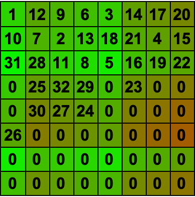
board = ReplacePart[ConstantArray[0, {8, 8}], {1, 1} -> 1];
solution =
DepthFirstSearch[board, iterateKnightWalk, (Max[#] == 32 &)];
If[solution =!= Nothing, finalBoard = Last[solution];
colorFunc[x_] :=
If[x == 0, White, Blend[{Green, Red}, x/Max[finalBoard]]];
styledBackground = Map[colorFunc, finalBoard, {2}];
labels = Map[Text[Style[#, Bold, 16]] &, finalBoard, {2}];
Grid[labels, Background -> styledBackground, Frame -> All],
Print["No solution found"]]
ClearAll[isPossible, solve];
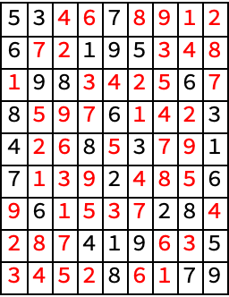
original = {{5, 3, 0, 0, 7, 0, 0, 0, 0}, {6, 0, 0, 1, 9, 5, 0, 0,
0}, {0, 9, 8, 0, 0, 0, 0, 6, 0}, {8, 0, 0, 0, 6, 0, 0, 0, 3}, {4,
0, 0, 8, 0, 3, 0, 0, 1}, {7, 0, 0, 0, 2, 0, 0, 0, 6}, {0, 6, 0, 0,
0, 0, 2, 8, 0}, {0, 0, 0, 4, 1, 9, 0, 0, 5}, {0, 0, 0, 0, 8, 0,
0, 7, 9}};
isPossible[sudoku_, y_, x_, n_] :=
And[FreeQ[sudoku[[y]], n], FreeQ[Transpose[sudoku][[x]], n],
FreeQ[Flatten[
Part[sudoku, 3 Floor[(y - 1)/3] + 1 ;; 3 Floor[(y - 1)/3] + 3,
3 Floor[(x - 1)/3] + 1 ;; 3 Floor[(x - 1)/3] + 3]], n]];
solve[sudoku_] /; ! MemberQ[Flatten[sudoku], 0] := sudoku;
solve[sudoku_] :=
Module[{emptyPos, y, x, n, newSudoku, result},
emptyPos = Position[sudoku, 0, 2, 1];
If[Length[emptyPos] == 0, Return[sudoku]];
{y, x} = First[emptyPos];
For[n = 1, n <= 9, n++,
If[isPossible[sudoku, y, x, n], newSudoku = sudoku;
newSudoku[[y, x]] = n;
result = solve[newSudoku];
If[result =!= Null, Return[result]];];];
Return[Null];];
solved = solve[original];
colorized =
MapThread[
If[#2 == 0, Style[#1, Red], Style[#1, Black]] &, {solved,
original}, 2];
Grid[colorized, Frame -> All]
Oh @Brad Klee I am so blessed to have been present for your divine implementation of the depth-first search function..and I know we were in a bit of a slump for a while there. You performed the backtracking, and you threw out a question about the improvements on previous backtracking algorithms..and now I think I finally understand why, because when you're navigating a chess knight across the board, you've got to iterate through possible states based on an iterator function. And by the time you check if a particular state is a solution, with the given function solutionQ, the possible states from our vantage point no longer exist from our perspective however they do exist within the DepthFirstSearch algorithm.
maze = {{1, 1, 1, 1, 1, 1, 1, 1, 1, 1, 1, 1, 1, 1, 1, 1}, {1, 0, 0, 0,
     0, 0, 0, 0, 0, 0, 0, 0, 0, 0, 0, 1}, {1, 0, 1, 1, 1, 1, 0, 1, 1,
    1, 1, 1, 1, 1, 0, 1}, {1, 0, 1, 0, 0, 0, 0, 1, 0, 0, 0, 0, 0, 1,
    0, 1}, {1, 0, 0, 0, 1, 1, 0, 1, 0, 1, 1, 1, 0, 1, 0, 1}, {1, 0, 1,
     0, 0, 0, 0, 1, 0, 0, 0, 1, 0, 1, 0, 1}, {1, 0, 0, 0, 0, 0, 0, 0,
    0, 0, 0, 0, 0, 1, 0, 1}, {1, 1, 1, 1, 1, 1, 1, 1, 1, 1, 1, 1, 1,
    1, 0, 1}, {1, 1, 1, 1, 1, 1, 1, 1, 1, 1, 1, 1, 1, 1, 0, 1}, {1, 0,
     0, 0, 0, 0, 0, 0, 0, 0, 0, 0, 0, 1, 0, 1}, {1, 0, 1, 0, 0, 0, 0,
    1, 0, 0, 0, 1, 0, 1, 0, 1}, {1, 0, 0, 0, 1, 1, 0, 1, 0, 1, 1, 1,
    0, 1, 0, 1}, {1, 0, 1, 0, 0, 0, 0, 1, 0, 0, 0, 0, 0, 1, 0, 1}, {1,
     0, 1, 1, 1, 1, 0, 1, 1, 1, 1, 1, 1, 1, 0, 1}, {1, 0, 0, 0, 0, 0,
    0, 0, 0, 0, 0, 0, 0, 0, 0, 1}, {1, 1, 1, 1, 1, 1, 1, 1, 1, 1, 1,
    1, 1, 1, 1, 1}};
moves = {{0, 1}, {1, 0}, {0, -1}, {-1, 0}};
DepthFirstSearch[maze_, start_, end_] :=
  Module[{stack = {}, visited = {}, position, path, next},
   AppendTo[stack, {start, {start}}];
   While[Length[stack] > 0, {position, path} = Last[stack];
    stack = Most[stack];
    If[Not[MemberQ[visited, position]], AppendTo[visited, position];
     If[position == end, Return[path],
      Do[next = position + move;
       If[
        1 <= next[[1]] <= Length[maze] &&
         1 <= next[[2]] <= Length[maze[[1]]] &&
         maze[[Sequence @@ next]] == 0 && Not[MemberQ[visited, next]],
         AppendTo[stack, {next, Append[path, next]}]], {move,
        moves}]]]];];
path = DepthFirstSearch[maze, {2, 2}, {15, 2}];
mazeWithSolution =
  If[path != {}, ReplacePart[maze, Thread[path -> 2]], maze];
MatrixForm /@ {maze, mazeWithSolution};
colorFunction[val_] :=
  Which[val == 1, Black, val == 0, White, val == 2, Red];
ArrayPlot[maze, ColorFunction -> colorFunction]
ArrayPlot[mazeWithSolution, ColorFunction -> colorFunction]

What about navigating a chess knight across an NxN grid? The moves a chess knight can make are defined, in the short term. An iterator - IterateKnightWalk - allows us to turn the knight on an NxN grid, and we switch around the results. That's the randomness, that's added to the iterator and ensures that each search run could rotate the results within the original framework turning an experimental disadvantage into an advantage; finding a Hamiltonian cycle for a knight on an 8x8 board is challenging, but a 6x6 board has better prospects. What kind of prospects? With regard to Directed Acyclic Graphs, the flexibility of the algorithm is showcased by applying it to even arbitrary Directed Acyclic Graphs. The function ToDirectedAcyclicGraph showcases how we can migrate and search through nodes of this graph, random or not. What do we do now?

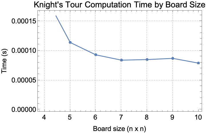
results = {};
Do[timing =
   AbsoluteTiming[
     DepthFirstSearch[
      ReplacePart[ConstantArray[0, {n, n}], {1, 1} -> 1],
      Function[IterateKnightWalk[#]], (Max[#] == n*n &), 1]][[1]];
  AppendTo[results, {n, timing}], {n, 4, 10}];
ListLinePlot[results, AxesLabel -> {"Board size (n x n)", "Time (s)"},
  GridLines -> Automatic, PlotTheme -> "Detailed",
 PlotStyle -> {Thickness[0.005]}, PlotMarkers -> Automatic,
 PlotLabel -> "Knight's Tour Computation Time by Board Size",
 Frame -> True, FrameLabel -> {"Board size (n x n)", "Time (s)"},
 LabelStyle -> Directive[Black, 12]]
When we apply BacktrackSearch on the demonstrations, I cannot calm down. I really appreciate the discussion of the results presented, I used to think results just grew on trees but then the orchestration of the chess knight problem really got us to a comprehensive understanding of the function's capabilities. I really hope that all of us users who are familiar with Wolfram technologies will not just lay low because we can't & want to refine a backtracking search function for Wolfram Mathematica. What is that? Backtracking is a general algorithm for finding solutions to some constraint satisfaction problems. It incrementally builds candidates to the solutions, and as soon as it determines that the candidate cannot be extended to a valid solution, the algorithm decisively backtracks on the candidate's journey laying low within the search space at each level.
$knightMoves = {{-2, -1}, {-2, 1}, {-1, -2}, {-1, 2}, {1, -2}, {1,
2}, {2, -1}, {2, 1}};
createKnightGraph[n_] :=
Flatten[Table[
If[And[i + #1 <= n, j + #2 <= n, i + #1 > 0, j + #2 > 0],
UndirectedEdge[{i, j}, {i + #1,
j + #2}]] & @@@ $knightMoves, {i, n}, {j, n}], 1];
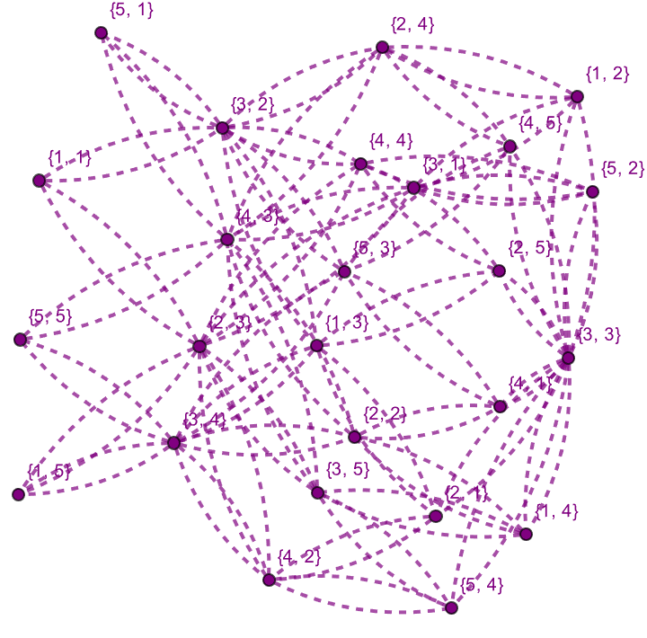
knightGraph = createKnightGraph[5];
validMoves = Select[Flatten[knightGraph], # =!= Null &];
GraphPlot[validMoves, VertexLabels -> Automatic,
PlotStyle -> Directive[Thick, Blend[{Red, Blue}, 0.5], Dashed]]
SeedRandom[123];
GenerateGraphData[edgesMultiplier_] :=
Table[g = RandomGraph[{size, edgesMultiplier*size}];
gDirected = ResourceFunction["ToDirectedAcyclicGraph"][g, 1];
edgeUpdate =
Association[# -> VertexOutComponent[gDirected, #, {1}] & /@
VertexList[gDirected]];
{size,
First@AbsoluteTiming@
DepthFirstSearch[1, edgeUpdate, (True &)]}, {size,
Range[10, 300, 10]}];
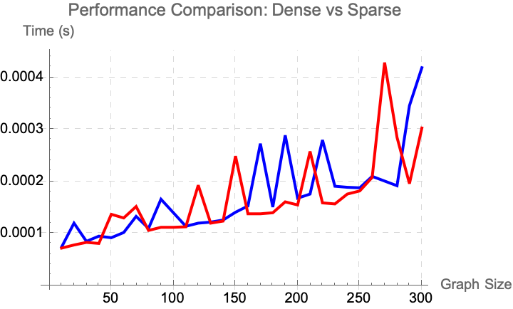
resultsDense = GenerateGraphData[3];
resultsSparse = GenerateGraphData[1];
ListLinePlot[{resultsDense, resultsSparse},
PlotLegends -> {"Dense", "Sparse"},
PlotStyle -> {Directive[Thick, Blue], Directive[Thick, Red]},
AxesLabel -> {"Graph Size", "Time (s)"},
PlotLabel -> "Performance Comparison: Dense vs Sparse",
GridLines -> Automatic,
GridLinesStyle -> Directive[LightGray, Dashed]]
The implementation search space and history just barely accommodates the problems where the potential states in the search space potentially depend on the entire history up to that point. The knight's tour problem asks if a knight on a chessboard can visit every square without repetition. The more general Hamiltonian path problem addresses these different data accordingly. The complexity of the knight's tour problem moves back from the presented data; there were only a few instances where a near-complete tour was found..and I want to do it too in a reasonable time. While the knight's tour problem serves as a good test for the algorithm, we should find some Directed Acyclic Graph. The advantage of such graphs is that it's computationally cheap because there are directed edges (arcs) with no cycles so there's always a topologically linear ordering of the vertices such that for every directed edge from vertex A to vertex B, A comes before B in the ordering.
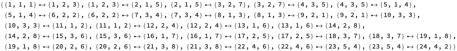
edges = Flatten[
Table[DirectedEdge[Position[solution, i][[1]],
Position[solution, i + 1][[1]]], {i, 1, 24}]]
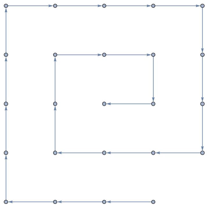
modifiedEdges =
DeleteCases[edges, {1, 1, 1} \[DirectedEdge] {1, 2, 3}];
Graph[modifiedEdges]
We found such significant content that we didn't even find more efficient self-reproductive strategies like breadth-first search (BFS)...depth-first search is in many cases computationally expensive due to its nature of exploring as far as possible along the tree of life before backtracking. The DFS backtracking algorithm can be visualized as a herd of animals for the purpose of optimization; for instance, using heuristics to guide the search - there's really just one search - or employing pruning techniques to eliminate false starts that are unlikely to lead to a solution...it's a formidably sublime approach to explore graphs where no two adjacent countries have the same color, we could probably even apply this to the leaf project. For instance, the decision where the daisy sprouts come out is determined by the concentration of plant hormone. We could probably handle arbitrary DAGs and Iterators to get a more tree-like structure. Anyway.
BFS can be computationally demanding to the large branching factor in the middle of the search. Again, BFS has the advantage of finding the shortest path from the starting position to any given target position on the board! Rather than finding a full knight's tour. It's sort of like growing some kind of cone cell in our eyes you've got to wire yourself up like BFS with the large number of possible board configurations: the depth-first nature tries to cover the board more extensively. It's like the Hiragana script, the possible moves of a knight as a tree or graph are neither skewed nor balanced in the conventional sense; the maximum breadth is 8, and the tree is so deep in terms of the sequences of moves that span the board; from the four central squares a knight can potentially reach every other square on the board in 6 moves..the maximum for the worst-case scenario.


