When you see our turned, sacred tree diffing, we can also generate some computational equations with a graphical interface for the differentiation, with the scale & range. Arnab, Tai, Zhang & Sasha we can also generate some phosphorescent geometric patterns for the minimum cost operation. Holy Shmoley there are so many LMDs. These are some of the all-time greatest dynamic programming algorithms.
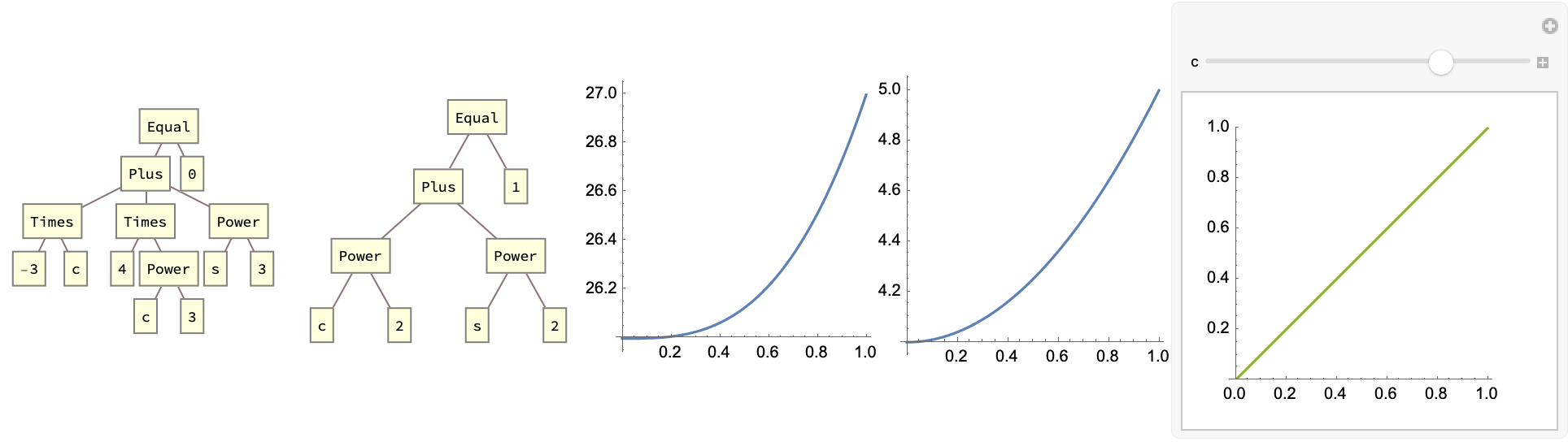
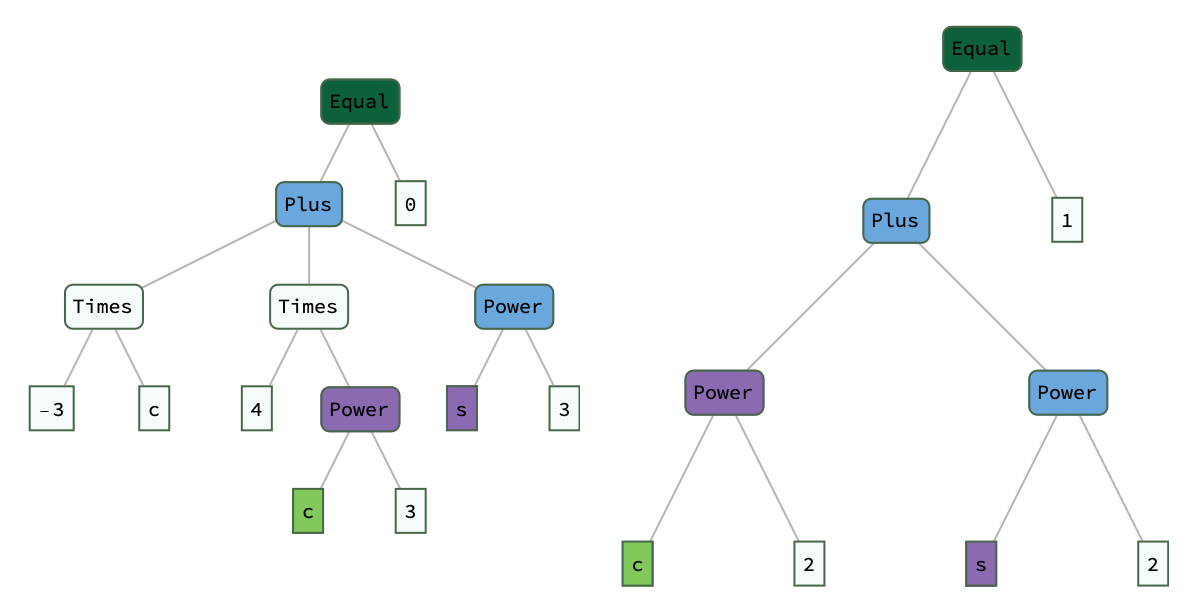
Subscript[eqn1, c_][s_] := -3 c + 4 c^3 + s^3
Subscript[eqn2, c_][s_] := c^2 + s^2
tree1 = TreeForm[eqn1, ImageSize -> Small];
tree2 = TreeForm[eqn2, ImageSize -> Small];
plot1 = Plot[Subscript[eqn1, 2][x], {x, 0, 1},
   AspectRatio -> Automatic, PlotRange -> Automatic,
   ImageSize -> Small];
plot2 = Plot[Subscript[eqn2, 2][x], {x, 0, 1},
   AspectRatio -> Automatic, PlotRange -> Automatic,
   ImageSize -> Small];
manipPlot =
  Manipulate[
   Plot[{Subscript[eqn1, c][s],
     Subscript[eqn1, c][Subscript[eqn1, c][s]], s}, {s, 0, 1},
    AspectRatio -> Automatic, PlotRange -> {0, 1},
    ImageSize -> Small], {{c, 3}, 0, 4}];
Row[{tree1, tree2, plot1, plot2, manipPlot}]
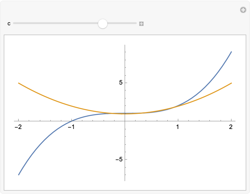
Manipulate[
 Plot[{-3 c + 4 c^3 + s^3, c^2 + s^2}, {s, -2, 2},
  PlotRange -> All], {c, -2, 2}]
There's a difference between two trees based on their structure & node labels? Really? Supposedly there's a minimum cost required to transform one tree into another. It's possible to draw parallels between tree diff'ing and DNA sequence alignment and yes the document formatting language is important. When you elaborate on the cost function associated with insert & delete it's like night and day. This is uniquely unparalleled research. This is the kind of research that Tai & Zhang do all the time. And they do it..because there's the essential, easily digestible enhancement..of the tree edit distance algorithm that calculates the distance between two trees by assessing how similar they are. But you know that already. The minimum number of operations - substitutions, deletions, insertions - required to transform one tree into another..it's such a succulent resource for postorder traversal matching of nodes transforming one tree to another type of list of operations that avoid repeated calculations by storing previous results in the td table, this is dense. Take this basic tree structure as far as it can achieve dynamic programming-wise, when I first saw this I didn't know what it was. Depending on the logic of the functions separation and the edit distance calculations, you might get any various kind of hierarchical data structure so go ahead.
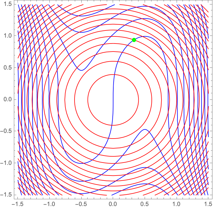
eqn1Func[c_, s_] := -3 c + 4 c^3 + s^3;
eqn2Func[c_, s_] := c^2 + s^2 - 1;
sol = FindRoot[{eqn1Func[c, s] == 0,
    eqn2Func[c, s] == 0}, {{c, 0.5}, {s, 0.5}}];
Show[ContourPlot[eqn1Func[c, s], {c, -1.5, 1.5}, {s, -1.5, 1.5},
  Contours -> 20, ContourShading -> None, ContourStyle -> Blue,
  PlotLegends -> Automatic],
 ContourPlot[eqn2Func[c, s], {c, -1.5, 1.5}, {s, -1.5, 1.5},
  Contours -> 20, ContourShading -> None, ContourStyle -> Red,
  PlotLegends -> Automatic],
 Graphics[{PointSize[Large], Green, Point[{c, s} /. sol]}]]
Change Detection in Hierarchically Structured Information you've been looking for Tai's method all along. You know who you are. In the meanwhile, the gap in existing literature is supposed to accentuate..the more traditional flat-file or sometimes relational data that has been the focus of prior works..users revisit pages on the World-Wide Web and want to understand changes since their last visit. The only reason I own the webpages is so that I can organize them, not to assume the existence of unique identifiers or keys to match the fragments of information that are scattered across versions and, in the real-life cases we achieve this musical orchestration where data doesn't come with identifying keys. When you bifurcate change detection, which apparently doesn't have any links to or references to the task at hand which is the transformation of ordered trees, the children of each node have a specific order; this is critical, because and after the two-fold subconcern of finding two good matchings and determining a minimum conforming edit script..@Arnab Datta you labeled what I could not, the Tai algorithmic, systematic objective criterion that mutates one tree to resemble another; nobody knew who he was. If that's what you really want, the paper puts a simple cost model with unit costs so you can delete while you insert, and insert while you move.
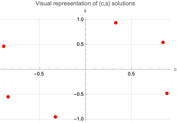
solutions = Solve[{eqn1, eqn2}, {c, s}];
ListPlot[{c, s} /. solutions, PlotStyle -> {Red, PointSize[Large]},
 AxesLabel -> {"c", "s"}, GridLines -> Automatic,
 PlotLabel -> "Visual representation of (c,s) solutions"]
operationVisualization[op_] :=
Module[{coloring},
coloring =
Switch[op[[1]],
"Delete", {Red, "Node " <> ToString[op[[2]]] <> " deleted"},
"Match", {Green,
"Node " <> ToString[op[[2]]] <> " matched with " <>
ToString[op[[3]]]},
"Substitute", {Orange,
"Node " <> ToString[op[[2]]] <> " substituted by " <>
ToString[op[[3]]]},
"Insert", {Blue, "Node " <> ToString[op[[2]]] <> " inserted"}];
{Graphics[{First@coloring, Disk[]}, ImageSize -> 20],
Last@coloring}];
visualizeTreeOps[treeA_, treeB_] :=
Module[{dist, op, visuals}, {dist, op} =
TreeEditDistanceOp[ExpressionTree[treeA], ExpressionTree[treeB]];
visuals = operationVisualization /@ op;
Grid[Prepend[visuals, {"Operation", "Description"}]]];
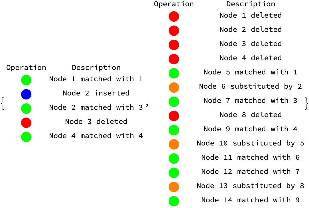
{visualizeTreeOps[{1, 2, 3}, {1, 3, 2}], visualizeTreeOps[eqn1, eqn2]}
How do you methodically break it down? Depending on the problems at hand, you might get a variety of edit scripts that approach comprehension, focus on the minimum cost for transforming one tree structure into another computative collective transform of treeA into treeB, the minimum conforming edit script. Children nodes from two matching nodes might be misaligned. The Longest Common Subsequence serves as the basis for the minimum number of moves for a real live alignment. And so the moves can delete, move, update, and insert nodes. It is so vivid, how the nodes from treeB are visited in a breadth-first order and depending on whether they have a partner in treeA, different actions are taken. Any nodes in treeA who didn't find a partner in treeB are removed. The isomorphic match of nodes between the two trees when the trees represent data without clear identifiers, promises more robust matching criteria, and it's never something that can be ever categorized so to speak; for leaf nodes and end nodes to be matched, they must have the same label and their values must be similar within the given threshold, of life. For internal nodes to be matched, they must have a substantially significant number of common leaf nodes. There are layers upon layers of labels that follow a certain order, and this is the moment we've been waiting for.
eqn1 = -3 c + 4 c^3 + s^3;
eqn2 = c^2 + s^2 == 1;
{distance, operations} =
  TreeEditDistanceOp @@ (ExpressionTree /@ {eqn1 == 0, eqn2});
ShowMatch @@ Join[ExpressionTree /@ {eqn1 == 0, eqn2}, {operations}]
Print[Evaluate@{eqn1 /. {c -> 2, s -> 1},
    Integrate[eqn1 /. {c -> 2, s -> 1}, {c, -1, 1}]}];
It's the icebreaker; the labels in the tree data should follow a certain order to ensure and then the structure can be represented without cycles. But is that true? The comparison function is used to determine the similarity of leaf nodes..so that each leaf resembles an other leaf. Is it discriminative enough? Does it even need to be discriminative? You could turn this into a movie. The movement of nodes is being tracked suggesting that yes there is a cost associated with this operation. The assumption of zero cost transforms the trees and simplifies certain algorithm, and that's why the way we move our subtrees from one node to another node of the parent tree when we do our fastText and our FastMatch..post-process suboptimal solutions in La-Tex and HTML documents..and do it for the trees. Do it for the unmatched nodes that are processed, linearly to handle insert/delete and match, move and remove the FastMatch to find the weighted linear relationship in hierarchically structured, non-document LaDiff, and the tradeoff between optimality and efficiency what they call it these days.
editDistanceOps[s1_, s2_] :=
  Module[{l1 = Length[s1], l2 = Length[s2], dp, i, j, ops = {}},
   dp = Table[0, {l1 + 1}, {l2 + 1}];
   For[i = 1, i <= l1 + 1, i++, dp[[i, 1]] = i - 1];
   For[j = 1, j <= l2 + 1, j++, dp[[1, j]] = j - 1];
   For[i = 2, i <= l1 + 1, i++,
    For[j = 2, j <= l2 + 1, j++,
      dp[[i, j]] =
       Min[dp[[i - 1, j]] + 1, dp[[i, j - 1]] + 1,
        dp[[i - 1, j - 1]] +
         If[s1[[i - 1]] == s2[[j - 1]], 0, 1]]];];
   i = l1; j = l2;
   While[i > 0 && j > 0,
    If[dp[[i + 1, j + 1]] - 1 == dp[[i, j + 1]],
     AppendTo[ops, {"Delete", s1[[i]]}]; i--,
     If[dp[[i + 1, j + 1]] - 1 == dp[[i + 1, j]],
      AppendTo[ops, {"Insert", s2[[j]]}]; j--,
      If[s1[[i]] == s2[[j]], AppendTo[ops, {"Match", s1[[i]]}]];
      If[dp[[i + 1, j + 1]] - 1 == dp[[i, j]] && s1[[i]] != s2[[j]],
       AppendTo[ops, {"Substitute", s1[[i]], s2[[j]]}]];
      i--; j--]]];
   While[i > 0, AppendTo[ops, {"Delete", s1[[i]]}]; i--];
   While[j > 0, AppendTo[ops, {"Insert", s2[[j]]}]; j--];
   Reverse[ops]];
visualizeOpsList[opsList_] :=
 Module[{coloring, visuals},
  coloring[op_] :=
   Switch[op[[1]], "Match", {Green, "Match: " <> op[[2]]},
    "Delete", {Red, "Delete: " <> op[[2]]},
    "Insert", {Blue, "Insert: " <> op[[2]]},
    "Substitute", {Purple,
     "Substitute: " <> op[[2]] <> " -> " <> op[[3]]}];
  visuals =
   Table[{Graphics[{coloring[op][[1]], Disk[]}, ImageSize -> 20],
     coloring[op][[2]]}, {op, opsList}];
  Grid[Prepend[visuals, {"Operation", "Description"}]]]
str1 = "kitten";
str2 = "sitting";
opsList = editDistanceOps[Characters[str1], Characters[str2]];
visualizeOpsList[opsList]
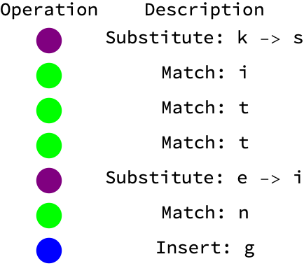
What questions haven't been answered? Can you read the code now? The edit distance between two strings s1 and s2, whichever the dp 2D array stores the operations, and it stores the minimum number of operations required to transform the substring s1[1...i] into s2[1...j]: it initializes the base case edit distance between an empty string and the first i characters of s1, & the first j characters of s2..the dp table is full of the edit distances between prefixes of strings s1 and s2, the dp[[l1+1, l2+1]] all possible prefixes based on one operation whether it's deletion dp[[i-1,j]]+1, insertion dp[[i,j-1]]+1; aren't the current characters s1[[i-1]] and s2[[j-1]] the same? The substitution cost of 1 or match cost of 0 - these base cases build up populate the dp table and backtrack to determine the exact operations that transform s1 to s2. The operations, are stored in the ops list; for each cell of dp the value is set to the minimum of the riveting, three operations - delete insert substitute & match.


