So like you suggest @Mark Merner we can provide a more general description of entanglement, than the classical. It could be the case that we would make up these axioms and every time we wanted to conclude something about mathematics we'd have to go down and be grunging around at the axiomatic level, that's not how mathematics actually works. The Bell test it's our experiment, it's our test of the predictions of quantum mechanics @Mark Merner against those of local realism, considering the possible configurations and variations of the QuantumToMultiwaySystem. I'm free to go over the mystical, this is so exciting! Consider the following. We certainly made it to measure the physical correlates of multiway diagrams, and the experimental mathematical axioms exist such that if we chose them then we wouldn't have a coherent view of mathematics; mathematics would kind of get shredded.
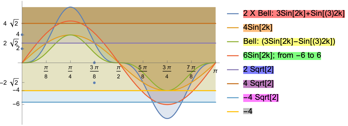
data = {{0, 2}, {0, 4}, {3 Pi/8, 0}, {3 Pi/8, -2 Sqrt[2]}};
plotData = {2 (3 Sin[2 k] - Sin[3*2 k]),
4 Sin[2 k], 3 Sin[2 k] - Sin[3*2 k],
6 Sin[2 k], 2 Sqrt[2], 4 Sqrt[2], -4 Sqrt[2], -4};
plotLegend = {Style["2 X Bell: 3Sin[2k]+Sin[(3)2k]",
Background -> RGBColor[1, 0, 0, 0.5]],
Style["4Sin[2k]", Background -> RGBColor[1, 0.5, 0, 0.5]],
Style["Bell: (3Sin[2k]-Sin[(3)2k])",
Background -> RGBColor[1, 1, 0, 0.5]],
Style["6Sin[2k]; from -6 to 6",
Background -> RGBColor[0, 1, 0, 0.5]],
Style["2 Sqrt[2]", Background -> RGBColor[0, 0, 1, 0.5]],
Style["4 Sqrt[2]", Background -> RGBColor[0.5, 0, 0.5, 0.5]],
Style["-4 Sqrt[2]", Background -> RGBColor[1, 0, 1, 0.5]],
Style["-4", Background -> RGBColor[0.5, 0.5, 0.5, 0.5]] };
plot = Show[
Plot[plotData, {k, 0, Pi}, Filling -> Top,
PlotLegends -> plotLegend],
ListPlot[data],
Ticks -> {{0.001 Pi, Pi/8, Pi/4,
3 Pi/8, Pi/2, 5 Pi/8,
6 Pi/8, 7 Pi/8, Pi},
{4 Sqrt[2], 2, 4, 2 Sqrt[2],
-2 Sqrt[2], -4, -6}}]
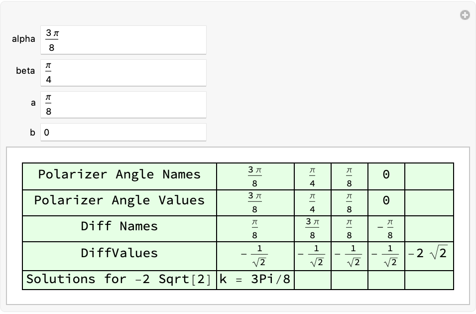
alpha = 3 Pi/8;
beta = Pi/4;
a = Pi/8;
b = 0;
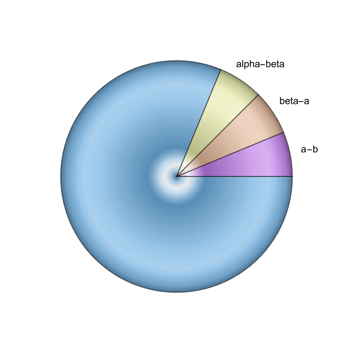
pieChart = PieChart[
{22.5, 22.5, 22.5, 292.5},
ChartLabels ->
Placed[{"a-b", "beta-a", "alpha-beta"}, "RadialOutside"],
SectorOrigin -> 0,
ChartElementFunction -> "GlassSector",
ChartStyle -> "Pastel"]
Manipulate[ClearAll[data, grid, diffNames, cosValues, S];
data = {{0, 2}, {0, 4}, {alpha, 0}, {alpha, -2 Sqrt[2]}};
diffNames = {alpha - beta, alpha - b, a - b, a - beta};
cosValues = {-Cos[2 (alpha - beta)], +Cos[2 (alpha - b)], -Cos[
2 (a - b)], -Cos[2 (a - beta)]};
S = Plus[-Cos[2 (alpha - beta)], +Cos[2 (alpha - b)], -Cos[
2*a - b], -Cos[2*(a - beta)]];
grid = Grid[
{{"Polarizer Angle Names", alpha, beta, a, b, ""},
{"Polarizer Angle Values", alpha, beta, a, b},
{"Diff Names", Sequence @@ diffNames, ""},
{"DiffValues", Sequence @@ cosValues, S},
{"Solutions for -2 Sqrt[2]", "k = 3Pi/8"}},
Background -> Hue[0.33, 1, 1, .1],
Frame -> All],
{alpha, 3 Pi/8, "alpha", 0, 2 Pi},
{beta, Pi/4, "beta", 0, 2 Pi},
{a, Pi/8, "a", 0, 2 Pi},
{b, 0, "b", 0, 2 Pi}]
There will be constraints, there may even be constraints we're seeing right now. There's a higher level experience of mathematics, it's kind of like we can experience not the molecules bouncing around in the room but the air currents. I love your color scheme and writing style let's steal some inspiration from the throes of your workflow.
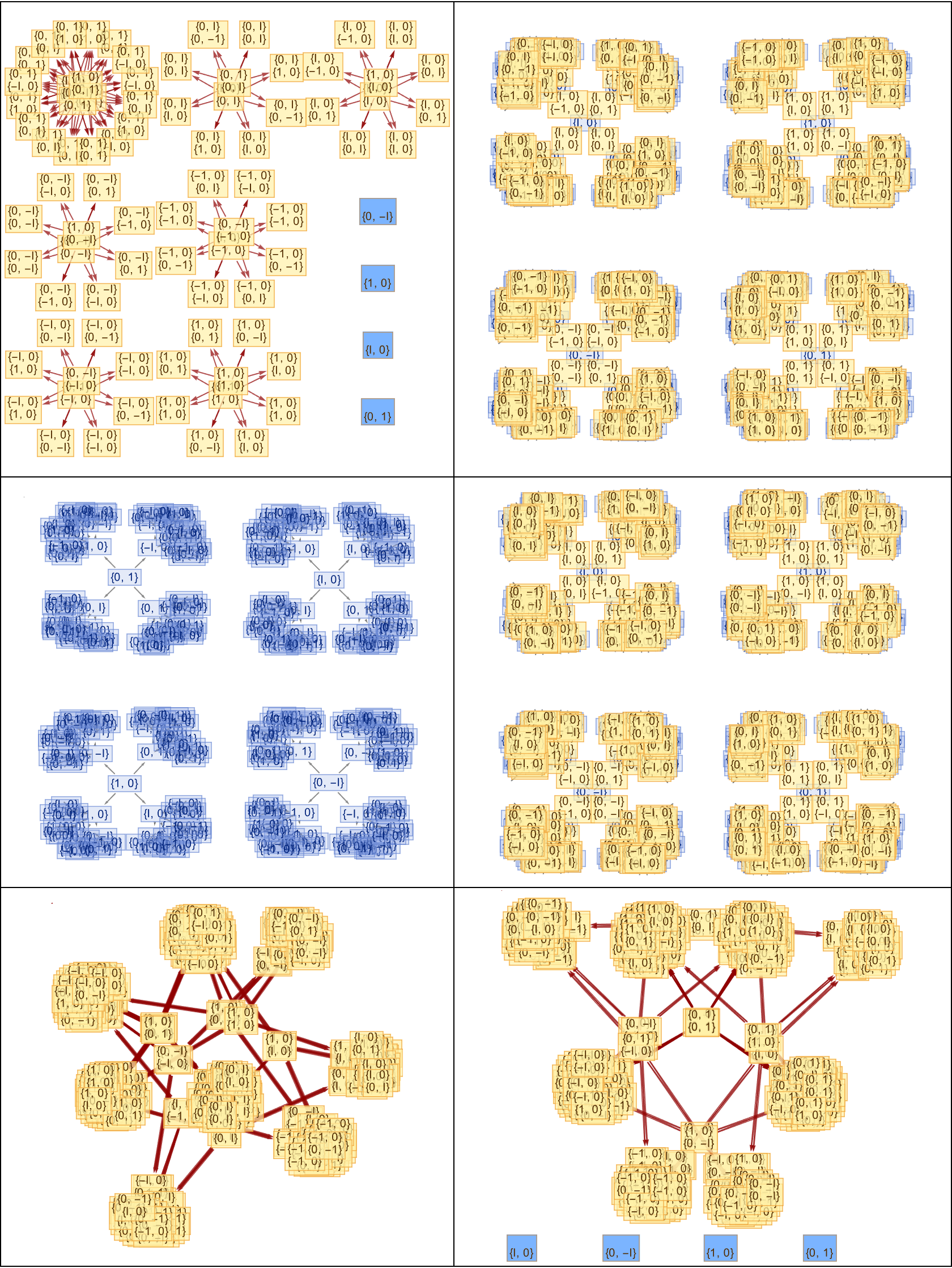
operator1 = {{1 + I, 1 - I}, {1 - I, 1 + I}};
operator2 = {{0, 1}, {1, 0}};
basis = {{1, 0}, {0, 1}};
initialState1 = {1 + I, 1 - I};
initialState2 = {0, 1};
steps = 3;
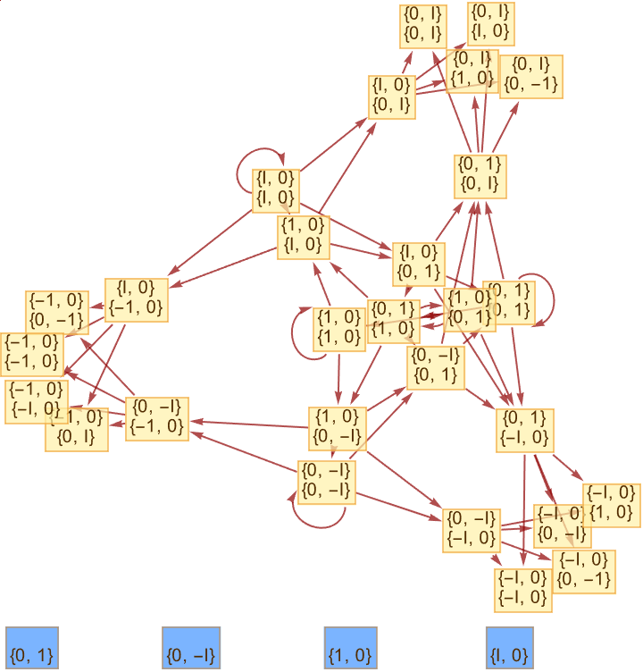
QuantumToMultiwaySystem[<|"Operator" -> operator1,
"Basis" -> basis|>, initialState1, steps, "StatesGraph",
"StateRenderingFunction" -> (RGBColor[RandomReal[], RandomReal[],
RandomReal[]] &)]
QuantumToMultiwaySystem[<|"Operator" -> operator1,
"Basis" -> basis|>, initialState1, steps, "CausalGraphInstances",
"MaxItems" -> 5]
QuantumToMultiwaySystem[<|"Operator" -> operator1,
"Basis" -> basis|>, initialState1, steps, "BranchPairsList",
"GivePredecessors" -> True]
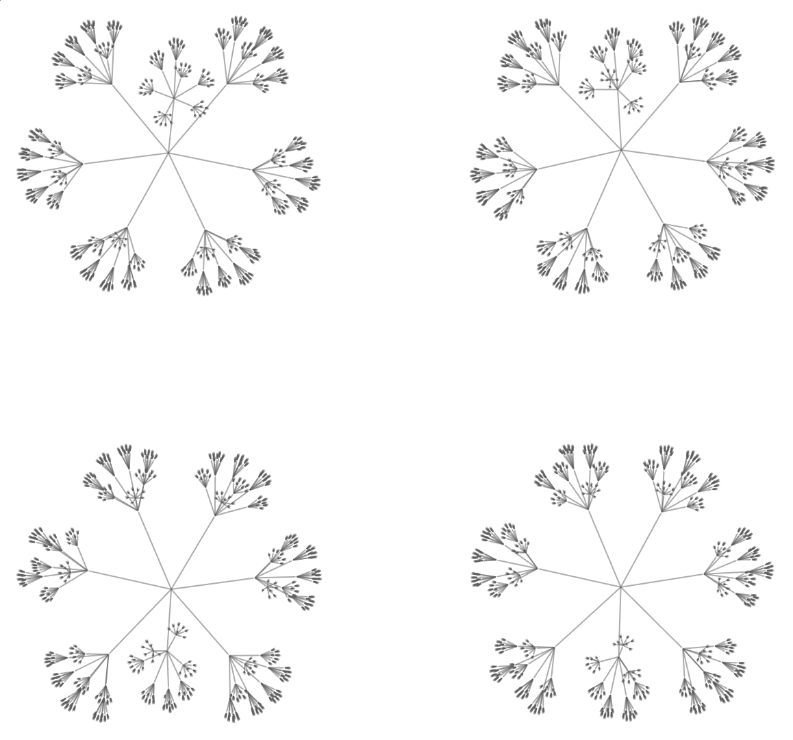
Table[QuantumToMultiwaySystem[<|"Operator" -> operator1,
"Basis" -> basis|>, initialState1, i, "StatesGraph"], {i, 0, 3}]
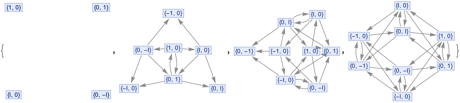
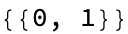
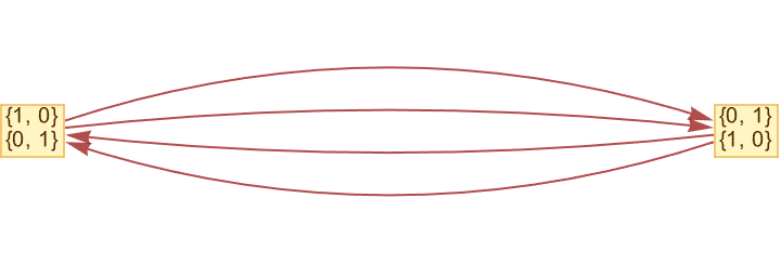
QuantumToMultiwaySystem[<|"Operator" -> operator2,
"Basis" -> basis|>, initialState2, steps]
QuantumToMultiwaySystem[<|"Operator" -> operator2,
"Basis" -> basis|>, initialState2, steps, "PredecessorRulesList"]
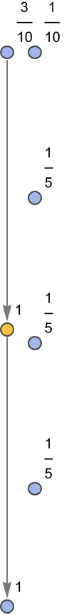
QuantumToMultiwaySystem[<|"Operator" -> operator2,
"Basis" -> basis|>, initialState2, steps, "EvolutionGraphWeighted"]
QuantumToMultiwaySystem[<|"Operator" -> operator2,
"Basis" -> basis|>, initialState2, steps, "StateWeights"]
QuantumToMultiwaySystem[<|"Operator" -> operator2,
"Basis" -> basis|>, initialState2, steps,
"IncludeStepNumber" -> True, "IncludeStateID" -> True]
QuantumToMultiwaySystem[<|"Operator" -> operator2,
"Basis" -> basis|>, initialState2, steps, "LineThickness" -> 2]
This photon polarization coincidence measurement reveals the distinct stages, between four or more detector pairs..it reminds me of that Crab Nebula in 1054, that was kind of hard to miss; there could be a supernova next week and we wouldn't know it. If we look at other galaxies we certainly see supernovas. But we can describe them in terms of simplicity and performance improvement because we've got the entanglement operators now. We can experience not the low-level sub-axiomatic foundations, but instead this kind of higher-level aesthetic thing that is the level that mathematicians typically experience things at. To what extent can we just go off and pick mathematics at random? @Mark Merner . These simulations of various experiments is like when William was going to England and when Halley was a statesman in the late 1600s, and that comet was named after him and one of those things that was of great interest was to explain them, how do orbits work?


These simulations could inform the design of real-world experiments to better understand the complex and subtle ways in which entanglement evolves. @Mark Merner A beta release is an initial release meant for a sub-set of users; maybe we can accomplish milestones successfully like the establishment of angle pairs, the measuring of causal invariance. What are these companies going to do, how are these technologies going to develop.


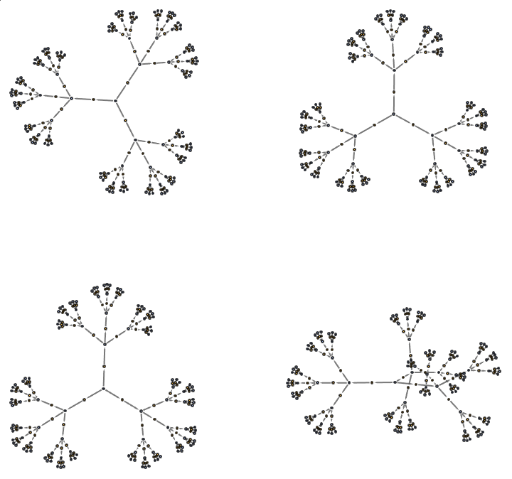
baseSteps[steps_, output_, options___] :=
  QuantumToMultiwaySystem[<|
    "Operator" -> {{1 + I, 1 - I}, {1 - I, 1 + I}},
    "Basis" -> {{1, 0}, {0, 1}}|>, {1 + I, 1 - I}, steps, output,
   "IncludeStepNumber" -> True, "IncludeStateID" -> True, options];

baseSteps[2, "AllEventsList"];
baseSteps[3, "CausalGraph", "IncludeInitializationEvents" -> True]
baseSteps[3, "EvolutionCausalGraph", "IncludeEventInstances" -> True]
baseSteps[3, "StatesGraph", "IncludeStateWeights" -> True]
baseSteps[3, "AllStatesList", "IncludeStatePathWeights" -> True];
baseSteps[2, "StatesCountsList"]
baseSteps[3, "CausalGraphInstances", "MaxItems" -> 5]
baseSteps[3, "EvolutionCausalGraph", "LineThickness" -> 2]
baseSteps[3, "CausalGraph", "IncludeInitializationEvents" -> True,
 "IncludeEventInstances" -> True]
baseSteps[2, "AllStatesList",
 "StateRenderingFunction" -> (Style[#1, Red] &),
 "EventRenderingFunction" -> (Style[#1, Blue] &)]
baseSteps[2, "AllStatesList", "GivePredecessors" -> True,
 "GiveResolvents" -> True]
baseSteps[3, "CausalGraph", "IncludeSelfPairs" -> True]
baseSteps[3, "CausalGraph", "IncludeFullBranchialSpace" -> True]
baseSteps[3, "CausalGraph", "LineThickness" -> 3]
Let's look at an analogy! @Mark Merner People had had electricity for 60 years and always thought it would be possible to transmit the human voice through an electrical line and hear it on the other end, but only when Alexander Graham Bell came along in 1874 did that actually work. The herd of scientific belief went in the direction of complete nonsense and I think we see that in all sorts of places where, oh Mark, I've been deeply involved in them; the continuity of space. Space is continuous.

Using the QuantumToMultiwaySystem in a high-dimensional (11D) setting, we've got to specify the operators & basis, to be used. The 5 Sigma Wigner Experiment, originally conducted by the Proietti group in Europe and the Bong group in Australia, tested the intriguing concept of Wigner's friend paradox!
Curry-Howard-Lambek + Church-Turing-thesis..does that make all proofs physical? Yes, it's an isomorphism that has the potential; make all proofs physical, simulate and visualize quantum processes in multi-dimensional spaces. The causal graph explores the strange nature of measurement in quantum mechanics. Charm Quarks & Anti-Charm Quarks; what's in-between them?
withStepState[operator_, basis_, initState_, steps_, output_,
   options___] :=
  QuantumToMultiwaySystem[<|"Operator" -> operator, "Basis" -> basis|>,
    initState, steps, output, "IncludeStepNumber" -> True,
   "IncludeStateID" -> True, options];
withStepState[{{1, 1 + I}, {1 + I, 1}}, {{0, 1}, {1, 0}}, {1 + I,
  1 - I}, 4, "EvolutionCausalGraphStructure",
 "IncludeStateWeights" -> True]
withStepState[{{0, 1}, {1, 0}}, {{1, 0}, {0, 1}}, {1,
  0}, 6, "EvolutionGraph"]
withStepState[{{1, 1 + I}, {1 + I, 1}}, {{0, 1}, {1, 0}}, {1 + I,
  1 - I}, 4, "CausalGraphInstances", "MaxItems" -> 15]
quantumFunc[operator_, basis_, initState_, steps_, output_,
   options___] :=
  Module[{processedOperator},
   processedOperator = ConjugateTranspose[operator . operator];
   withStepState[processedOperator, basis, initState, steps, output,
    options]];
quantumFunc[{{1, 1 + I}, {1 + I, 1}}, {{0, 1}, {1, 0}}, {1 + I,
  1 - I}, 4, "StatesGraphStructure", "IncludeStateWeights" -> False]
This is even stranger than the strangest nature of measurement, that is in quantum mechanics. Physical processes occurring at one location do not depend on the properties of objects at other locations; they absolutely did not know it was a star exploding. "Causal invariants", are mathematical objects that stay the same under a specific set of transformations. That is the result of the simulation that is the concept of what physical processes really go on in the six entanglement simulations. Four of them correspond to a Bell test, and two lines correspond to communications, with Wigner's friends.


withOperatorBasis[output_, options___] :=
  QuantumToMultiwaySystem[<|"Operator" -> {{0, 1}, {1, 0}},
    "Basis" -> {{1, 0}, {0, 1}}|>, {0, 1}, 5, output, options];
withOperatorBasis["CausalGraph", "IncludeEventInstances" -> True]
withOperatorBasis["CausalGraph", "IncludeStepNumber" -> True,
 "IncludeStateID" -> True]
withOperatorBasis["EvolutionEventsGraph", "IncludeStepNumber" -> True,
  "IncludeStateID" -> True]
With regard to the photons, the physical correlates of quantum multiway diagrams in nature, like when the sun got covered, and everybody freaked out they ran away from the battle..we could turn off the entanglement between Wigner and his friends. I would not be surprised that Thales and Ptolemy knew about that all along! The Antikythera, people would prove the best theorems about astronomy.


operator = {{0, 1, -Cos[2 ((2 \[Pi])/8 - (1 \[Pi])/8)], 1, 0},
   (1 + I)/Sqrt[2] {0, 1, -Cos[2 ((2 \[Pi])/8 - (0 \[Pi])/8)], 1, 0},
   {1, 0, 1, 1, 1},
   {1, 0, -Cos[2 ((0 \[Pi])/8 - (0 \[Pi])/8)], 1, 0},
   (1 + I)/Sqrt[2] {0, 1, -Cos[2 ((0 \[Pi])/8 - (1 \[Pi])/8)], 1,
     0}};
basis = {{1, 1, 1, 1, 1},
   {0, 1, 1, 1, 1},
   {0, 0, 1, 1, 1},
   {0, 0, 0, 1, 1},
   {0, 0, 0, 0, 1}};
initState = {{1, 0, 1, 1, 1},
   {0, 1, 1, 1, 1} - {0, 0, 1, 1, 0},
   {0, 1, 1, 1, 1}};
timeFn[tRange_, output_, options___] := AbsoluteTiming[Table[
    QuantumToMultiwaySystem[<|"Operator" -> operator,
      "Basis" -> basis|>, initState, t, output, options],
    {t, tRange}]];
timeFn[1, "EvolutionCausalGraphStructure",
 "IncludeStateWeights" -> True, VertexLabels -> "VertexWeight"]
timeFn[1, "EvolutionCausalGraphStructure",
 "IncludeStateWeights" -> True, VertexLabels -> "VertexWeight",
 "IncludeStepNumber" -> True, "IncludeStateID" -> True]
QuantumToMultiwaySystem[<|"Operator" -> {{0, 1}, {1, 0}},
  "Basis" -> {{1, 0}, {0, 1}}|>]
Our new generation of Sigma5 level type inequality experiments, also known as the Wigner's Friends experiments, are freely accessible via the QuantumToMultiwaySystem tool. The rational unified phases, meta-linguistic awareness is the consciousness of forming languages which expresses memes transcending specific expression; in that sense we are aware of the distinct stages in the evolution and completion of quantum entanglement, with our photon polarization coincidence measurements. These approaches simulate various experiments informing the design of real-world experiments..how we understand the complex and subtle ways in which entanglement evolves. Everything is made out of water, maybe the world is made of discrete things like atoms.
data = QuantumToMultiwaySystem[<|
"Operator" -> {{1 + I, 1 - I}, {1 - I, 1 + I}},
"Basis" -> {{1, 0}, {0, 1}}|>,
{1 + I, 1 - I},
2,
"AllStatesList",
"IncludeStepNumber" -> True,
"IncludeStateID" -> True,
"StateRenderingFunction" -> Automatic,
"EventRenderingFunction" -> Automatic,
MaxItems -> 10];
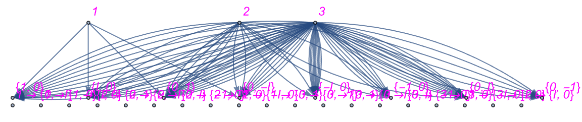
edges = Flatten[MapIndexed[Thread[First[#2] -> Values[#1]] &, data]];
vertices = Union[Flatten[edges]];
Graph[vertices,
edges,
VertexLabels -> "Name",
ImageSize -> Large,
VertexSize -> 0.4,
VertexLabelStyle -> Directive[RGBColor[1, 0, 1], Italic, 12]]
QuantumToMultiwaySystem[<|
"Operator" -> {{1 + I, 1 - I}, {1 - I, 1 + I}},
"Basis" -> {{1, 0}, {0, 1}}|>,
{1 + I, 1 - I},
2,
"CausalGraph",
"IncludeInitializationEvents" -> True,
"IncludeEventInstances" -> True]
The Guest star, what was it? At the hands of the Catholic Church actually, yes, the stars are like the sun but far away. I suppose it's really the exploration of quantum entanglement that gets us where we need to be. When I read your article, I was so emotionally starstruck that I was unable to introduce the concept of an entanglement life cycle like you did.