Yea, find some positive integer sequences for a beautiful, technical, and comparative Wolfram Annual Summit! Bring up the notion of sequences, we don't have - we do have enough computational space to go all the way "back" to the beginning of a sequence? It's very simple. Unless your screen size is really big, which it is.

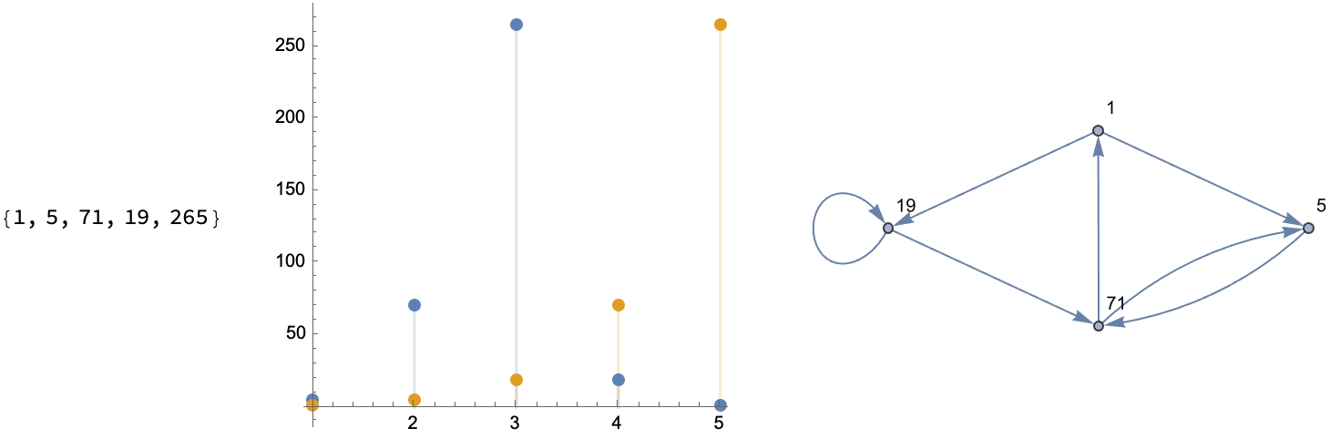
tab = 5;
2*RecurrenceTable[{a[n + 1] == 14*a[n] - a[n - 1], a[0] == 1, 
     a[1] == 1}, a, {n, 1, tab}] - 1; 
A = Sqrt[%];
For[i = 1, i <= Factorial[tab], i++,
 orb[i] = Take[Permutations[Range[tab]], Factorial[tab]][[i]]]
Do[(orbit = orb[k];
  len = Length[orbit];
  permList = PermutationList[Cycles[{orbit}]];
  seq = {};
  Do[AppendTo[seq, {i, permList[[i]]}], {i, 1, len}];
  f = Interpolation[seq, InterpolationOrder -> 1];
  edge = {};
  Do[Do[If[j >= Round[NMinValue[{f[x], i <= x <= i + 1}, x]] &&
      j + 1 <= Round[NMaxValue[{f[x], i <= x <= i + 1}, x]],
     AppendTo[edge, A[[i]] -> A[[j]]]], {j, len - 1}] , {i, 
    len - 1}];
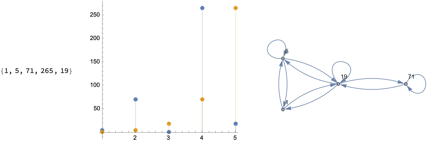
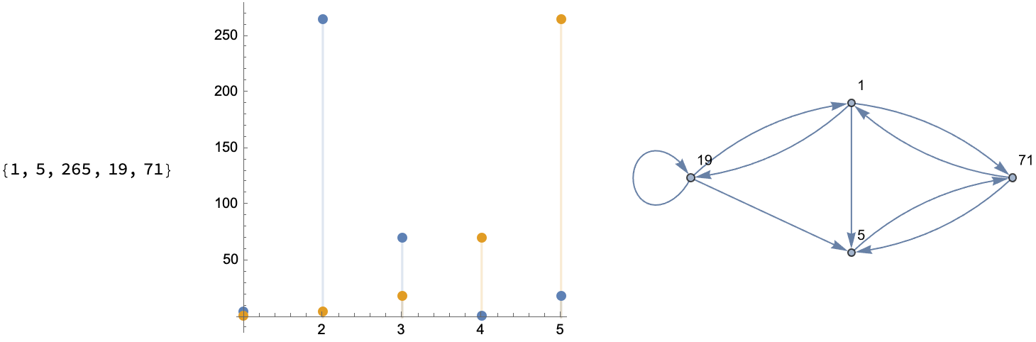
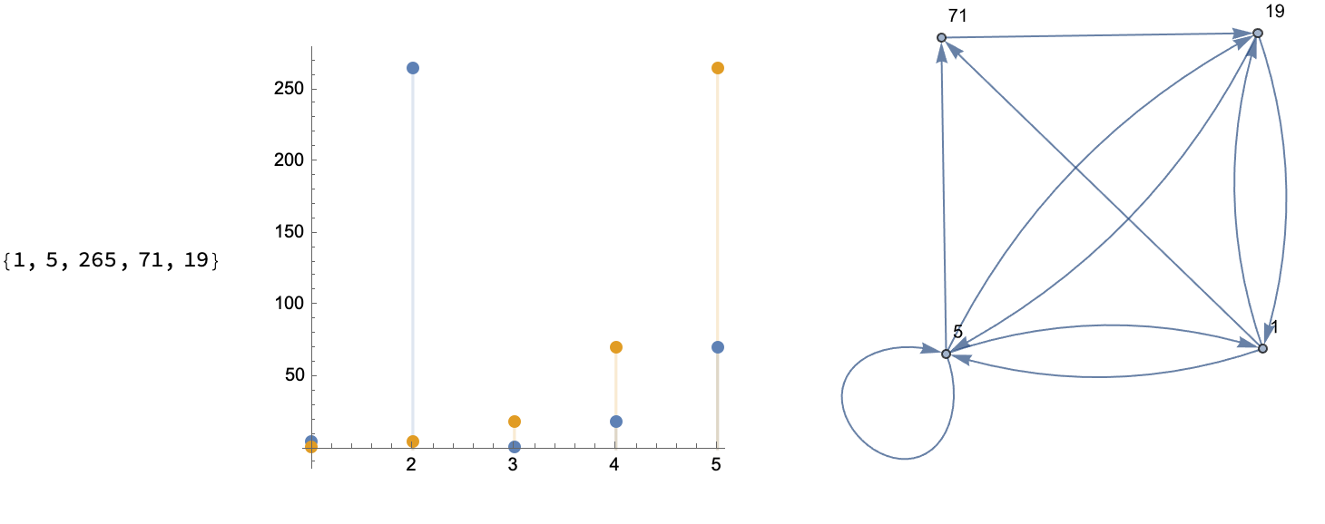
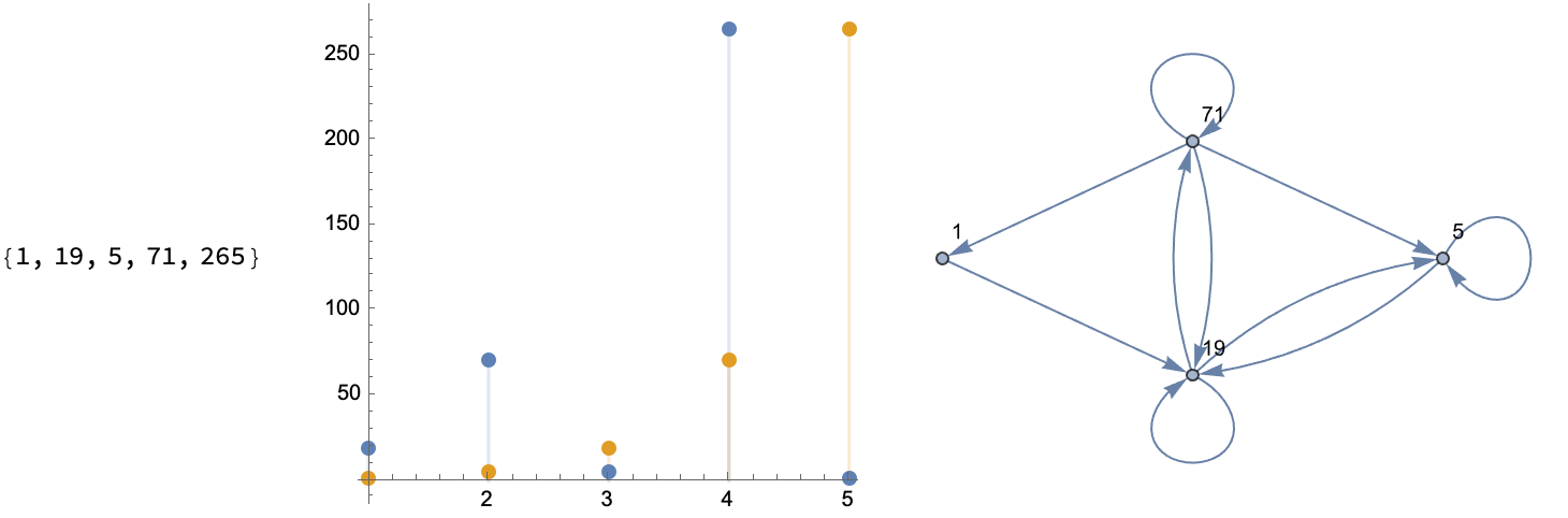
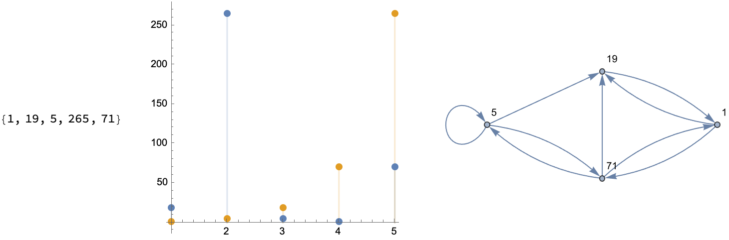
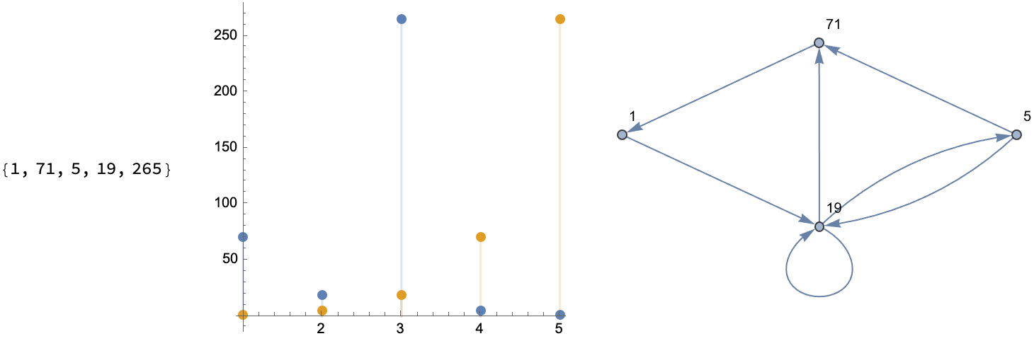
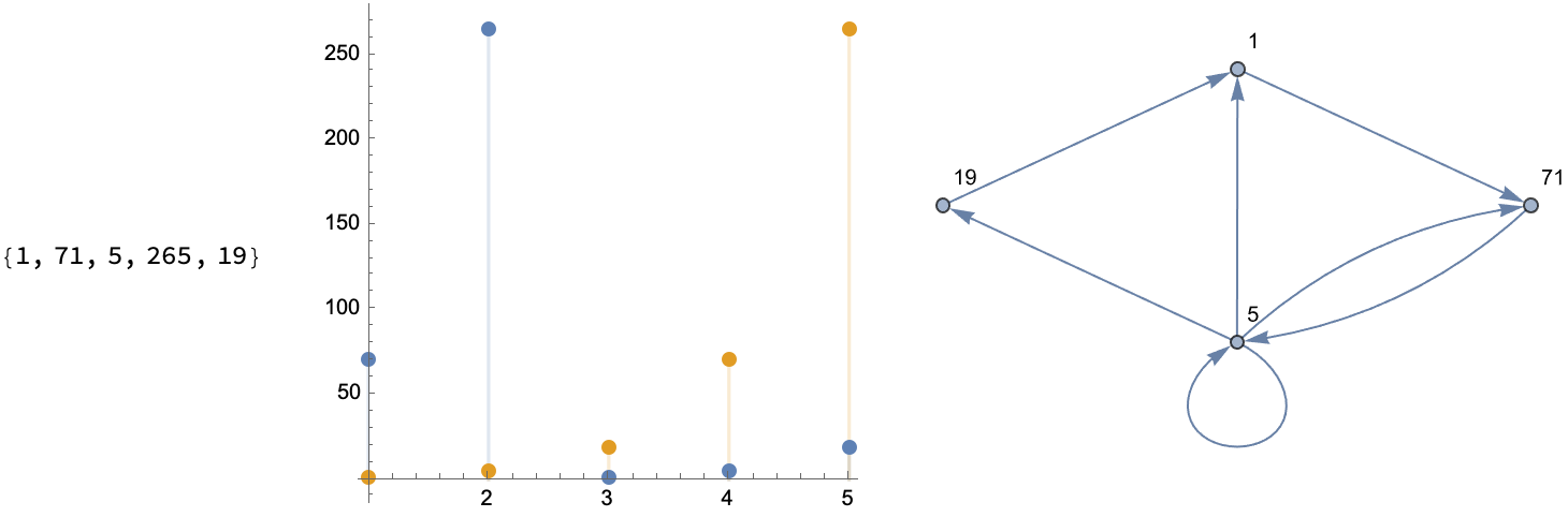
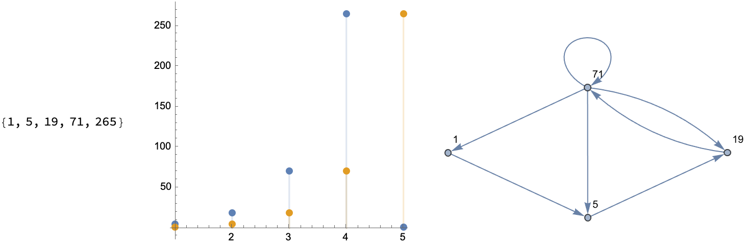
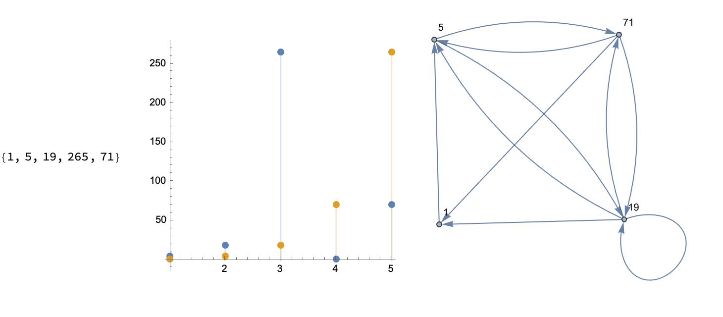
  Print[Row[{A[[orbit]], "    ",
      DiscretePlot[{A[[Round[f[x]]]], A[[Round[x]]]}, {x, 1, len}, 
      AspectRatio -> 1, PlotStyle -> PointSize[0.03], 
      ImageSize -> 250], "    ",
      Graph[edge, VertexLabels -> Automatic, 
      ImageSize -> 300]}]]), {k, Factorial[tab]}]

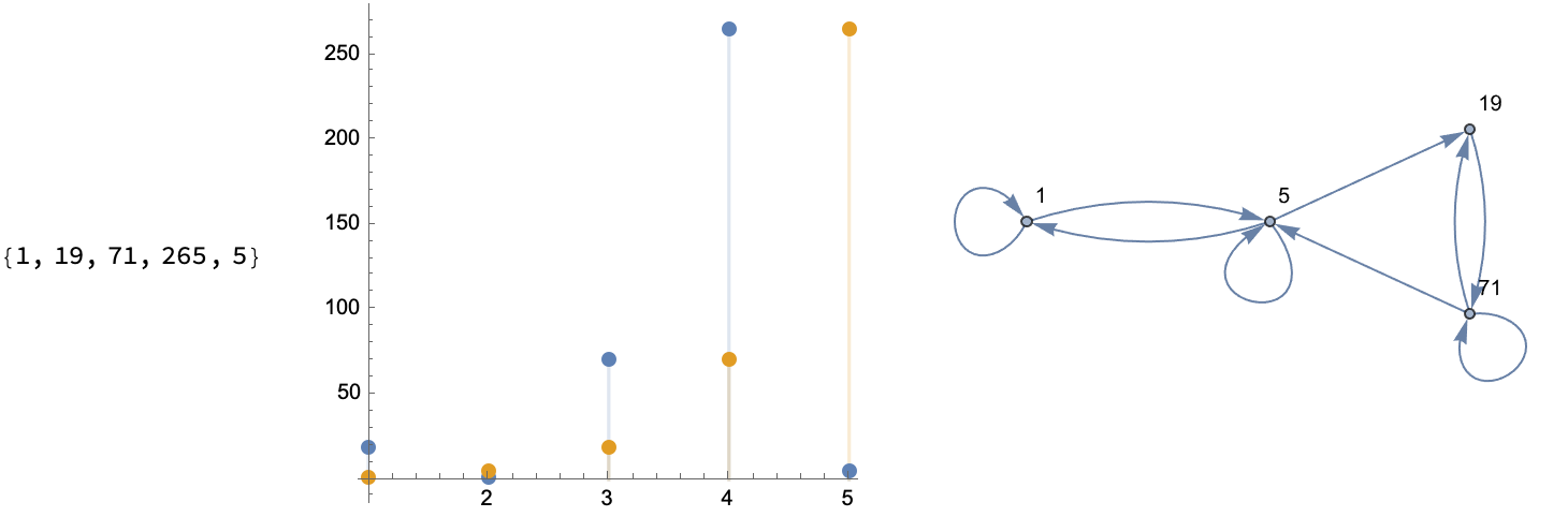
What kind of graph do you want to look at, to understand sequences? You could have a permutation like {1, 2, 3, 5, 4} and then form an orbit, like the one we start at and arrive at some sliding window via some scalar InterpolatingFunction, on the order of 1. And then step up through the values to Do an outer "loop" of rows.

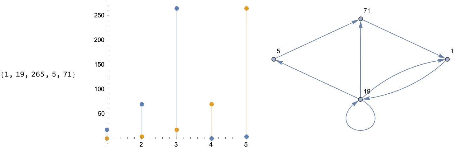
How do you add more tick marks and customize these graphs, which show us the index whether it's a time series or some scatterplot like what we can make, yes we can enjoy the festivities and draw a line and then make some DiscretePlot.. yikes!

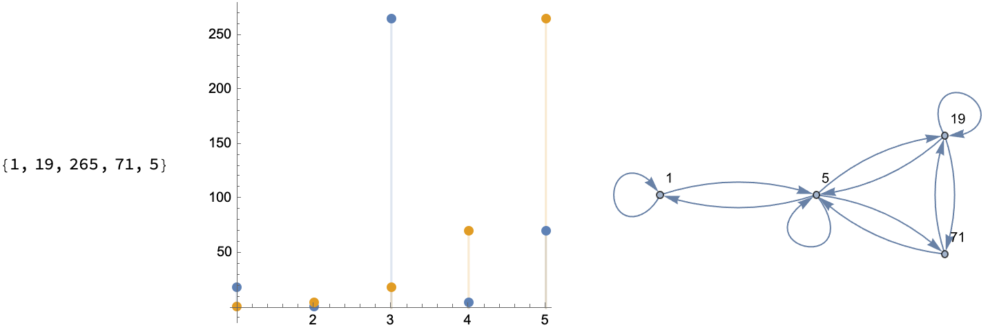
Then, maybe our initial assumptions were wrong so we double under-line, to get some perfect, linearly recurring sequence & graphs. And what do you get? 1, 1, 25, 361..., so that you can do recursion and see the permutation progression of these sequences. Tada!

I think that part of the thing is that when you're designing these archives of mathematical Olympiad problems they're supposed to both be suitable for both manual and computational exploration, via the Wolfram Language. And it's really for people like Ramanujan and those among us, who has such an infectious personality. This methodology that you've developed shows us how to spearhead the initiative, and make things possible that were never possible before. Now, we can generate geometry problems and things that already exist or may not have existed yet, and I have absolutely no idea what kind of Euclidean Geometry problems are going to come up. But what I do know is and this is my very first time, given that Mathematica is highly customizable, we're going to have this dichotomic thing where the educators, they see this absence of Euclidean Geometry problems and we can actually build them out in an easy to find archive of all that advice we've been saving, what with the running a physical server on Ubuntu and deploying my app that I built with xampp that has mysql db's as well with a lot of dynamic content. Or, we could just build this project using the computational tools of Mathematica which is a valuable resource for students and enthusiasts in mathematical problem-solving.

fibonacciNumbers1200AD[0] = 0;
fibonacciNumbers1200AD[1] = 1;
fibonacciNumbers1200AD[n_] := 
  fibonacciNumbers1200AD[n] = 
   fibonacciNumbers1200AD[n - 1] + fibonacciNumbers1200AD[n - 2];
lucasRecurrence[0] = 2;
lucasRecurrence[1] = 1;
lucasRecurrence[n_] := 
  lucasRecurrence[n] = lucasRecurrence[n - 1] + lucasRecurrence[n - 2];
fibonacciPolynomial[0] = 0;
fibonacciPolynomial[1] = 1;
fibonacciPolynomial[n_] := 
  fibonacciPolynomial[n] = 
   2*fibonacciPolynomial[n - 1] + fibonacciPolynomial[n - 2];
fibonacciRecurrence = Table[fibonacciNumbers1200AD[n], {n, 0, 20}];
lucasRecurrence = Table[lucasRecurrence[n], {n, 0, 20}];
fibonacciPolynomialRecurrence = 
  Table[fibonacciPolynomial[n], {n, 0, 20}];
ListLinePlot[
 {fibonacciRecurrence, lucasRecurrence, fibonacciPolynomialRecurrence},
 PlotLegends -> {"Fibonacci Sequence", "Lucas Sequence", 
   "Fibonacci Polynomial Sequence, for x=2"},
 AxesLabel -> {"n", "Sequence Value"},
 PlotMarkers -> {"o", "s", "*"},
 GridLines -> Automatic,
 GridLinesStyle -> Directive[GrayLevel[0.5], Dashed]]

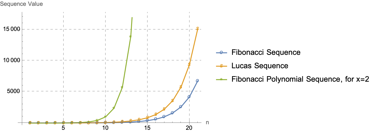
It would be interesting to get the Fibonacci sequence and significant work like Patrik Bak's automated generation of geometry problems, which already exists by the by, and this interface development which just serves as what we knew we had before..the only question is to ask what we had before and where we are going which is not anywhere, but it is something that we want to supplement traditional problem-solving techniques..it's the categorization, it really is like being in a cave I don't know how else to categorize these problems into areas such as Algebra, Number Theory, and Probability. Once I get started I tag them with difficulty levels from things like "easy" to.."hard". Then, we've got this timeless project of yours which seeks to enhance our problem-solving skills and discover the capabilities, and the limitations, of the Wolfram Language. I wonder if the development of these interfaces might serve as a primary focus at this stage, for proving the concept that we can have a beautiful database on archive, a Mathematical Olympiad problem database.

ParametricPlot[
 {Sin[t]*(Exp[Cos[t]] - 2 Cos[4 t] - Sin[t/12]^5), 
  Cos[t]*(Exp[Cos[t]] - 2 Cos[4 t] - Sin[t/12]^5)},
 {t, -Pi, Pi},
 PlotStyle -> {Thick, Black},
 AxesLabel -> {"Re(z)", "Im(z)"},
 LabelStyle -> 
  Directive[FontFamily -> "Helvetica", FontSize -> 14, Black],
 AxesStyle -> Thick,
 Frame -> True,
 FrameStyle -> Directive[Black, 12],
 GridLines -> Automatic,
 GridLinesStyle -> Directive[Gray, Dashed],
 PlotRange -> All, PlotRangePadding -> Scaled[0.05],
 ImageSize -> 500,
 PlotLegends -> Placed["Butterfly Curve", Below]
 ]

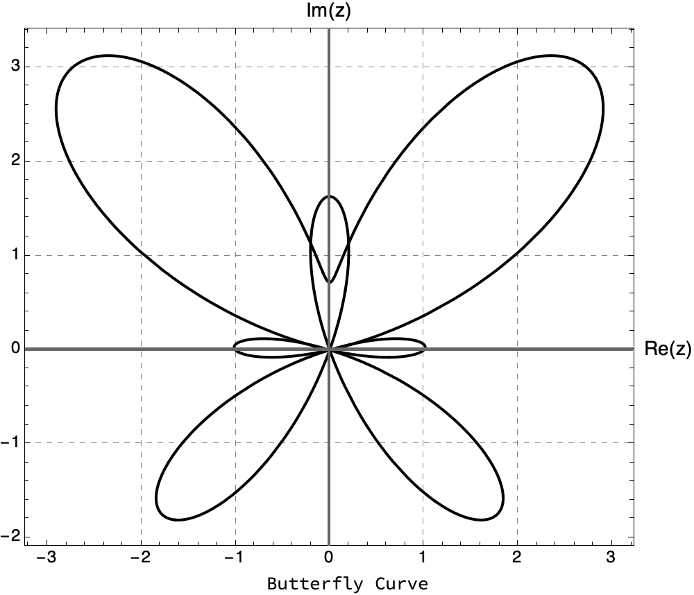
I believe the real question is, do I like this graph? To put it quite succinctly, I think there's a ton of dynamic content if you think of it as a butterfly, a shoelace, because once the Wolfram Language begins these sample problems it just has to illustrate from the Bulgaria Festival of Young Mathematicians, and showcase how we can make effective utilization of the Wolfram Language in order to find patterns in sequences, and prove patterns in sequences, which is important because it illustrates the practical application of the database. One thing I'd like to take a look at is something which I would categorize as part of this project: the advanced mathematical problem-solving techniques that have been made accessible and therefore provide an educational tool wherein we can make logistic maps. Let's take a look at this guy, go!

rValues = Range[2.5, 4, 0.0025];
lastIterations = 30;
transientIterations = 100;
a = 0.3; 
colorFunction = ColorData["RedBlueTones"];
logisticMapLensExtended = Flatten[
   Table[
    Module[{x = 0.5},
     Table[x = r x (1 - x) - a x^2, {transientIterations}];
     Table[{r, x, 
       colorFunction[Rescale[r, {2.5, 4}]]}, {lastIterations}]
     ],
    {r, rValues}
    ],
   1
   ];
Graphics[
 {
  PointSize[0.01],
  Point[{#[[1]], #[[2]]}, VertexColors -> #[[3]]] & /@ 
   logisticMapLensExtended
  },
 Axes -> True,
 AxesLabel -> {"r", "x"},
 PlotRange -> All
 ]

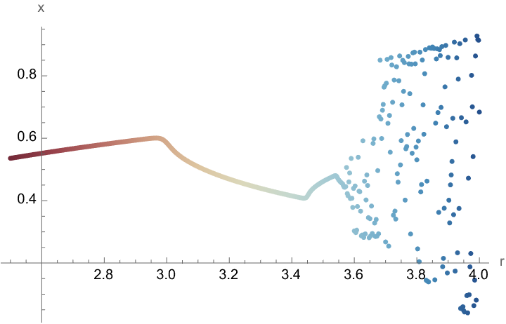
This logistic map shows how we can even make more advanced mathematical explorations, possibly at events..I'm only seeing the blue part of the graph and I don't know why, it's probably because we need more advanced computational resources to analyze the structure and behavior of sequences. I think that as a conclusion, we can classify the Wolfram Mathematical Olympiad problems database as one which has significant educational potential because that's how we can get things like a blend of computational and theoretical skills.

henonMap[a_, b_, {x0_, y0_}, n_] := 
  NestList[{1 - a #[[1]]^2 + #[[2]], b #[[1]]} &, {x0, y0}, n];
a = 1.4;
b = 0.3;
initialPoint = {0.1, 0.1};
iterations = 10000;
data = henonMap[a, b, initialPoint, iterations];
{xMin, xMax} = MinMax[data[[All, 1]]];
myColorFunction[x_] := 
  ColorData["RedBlueTones"][(x - xMin)/(xMax - xMin)];
coloredData = {myColorFunction[#[[1]]], Point[#[[1 ;; 2]]]} & /@ 
   data;
Graphics[{PointSize[0.01], coloredData}, Axes -> True, 
 AxesLabel -> {"x", "y"}, PlotRange -> All]

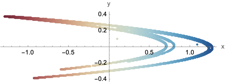
I think that the Henon map as a discrete-time dynamical system that serves as a simplified model of chaotic systems.. it's the type of system that we want to study all of the context of mathematical physics and dynamical systems theory, which me thinks could be of interest in an Olympiad setting when you're illustrating complex mathematical concepts. Personally, I think it could be a lot like discovering the Antikythera device in the exact same way, that we do natural language processing and we do, we take some parameters, define an initial point, and then iterate the map to produce the list of points. Do we set parameters for the Henon map to result in chaotic behavior? Do we generate the trajectory of the map over 10000 iterations? Yes, and the reason will be that initial conditions can evolve into a fractal-like pattern, which is a hallmark of chaotic systems. This is an advanced topic suitable for high-level mathematical competitions and education. It's like the light at the top of A New Kind of Science, it's similar to the uniformly symmetric dynamic of chaos theory and like any Olympiad project, for example these computational tools illustrate abstract concepts in a way that we can feel and hold.

paramSpace = Flatten[
   Table[
    {r, b, Last[NestList[(#^2 - b) &, 0.1, 50]]},
    {r, 0, 2, 0.1},
    {b, 0, 1, 0.05}],
   1
   ];
ListPlot3D[
 paramSpace,
 AxesLabel -> {"r", "b", "x"},
 ColorFunction -> "RedBlueTones",
 Mesh -> None,
 ColorFunctionScaling -> True
 ]

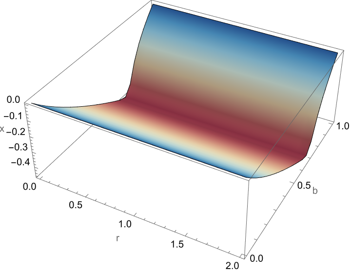
I don't know how many times I applied that function iteratively, the probability is that I applied it 50 times with an initial value of 0.1 and this is what allows us to generate this simplified one-dimensional map and thereby capture the end state of the dynamical system after 50 iterations, for each parameter combination. And with the dynamic of chaos theory, and the kind of parameter spaces in mathematical models you might find at a used book store, there's chaos theory and the exploration of it reveals how changing parameters affect the behavior of a system, which can lead to deeper insights or even just the low-hanging fruit regarding the system's stability, bifurcations, or onset of chaotic behavior.

lyapunovExponent[r_, n_] := Module[
   {x = 0.1, lyapunov = 0},
   Table[lyapunov += Log[Abs[r (1 - 2 x)]];
    x = r x (1 - x);, {n}];
   lyapunov/n];
data = Table[{
    r,
    lyapunovExponent[r, 1000]
    },
   {r, 2.5, 4, 0.001}];
lyapunovValues = data[[All, 2]];
minLyapunov = Min[lyapunovValues];
maxLyapunov = Max[lyapunovValues];
colorFunction = ColorData["RedBlueTones"];
ListPlot[
 data,
 Joined -> True,
 PlotStyle -> PointSize[1.00],
 ColorFunction -> (colorFunction[#2] &),
 ColorFunctionScaling -> True
 ]

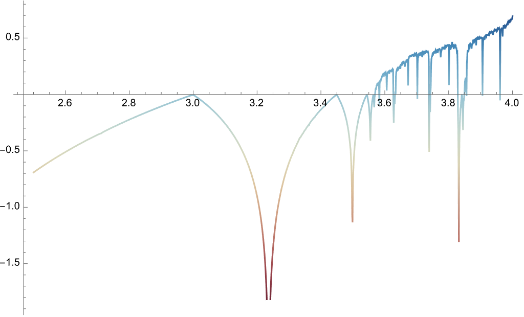
I think that the concept of parameter spaces and their impact on system dynamics, is like those Egyptian receipts for barley in that we can use computational tools in mathematical research, which allows for complex systems to be simulated and analyzed efficiently and having this database is sort of like having Cleopatra and Marc Antony in the same room, it's especially relevant given the rise of computational mathematics and its applications in problem-solving and research, which brings up how we can compute and plot this Lyapunov exponent in a logistic map. This is a simple model for chaos, which accumulates the log of the absolute value of the derivative and thereby divides the sum by n to normalize the exponent over the number of iterations, and represent the behavior of the logistic map at the value r, after 1000 iterations. So after all those iterations, we can visualize the transition from stable to chaotic behavior in a dynamical system as the parameter r changes. I hope that this visual representation serves as a source of warmth for Olympiad students studying complex systems or non-linear dynamics. But what it does do is, the Lyapunov exponent is a quantitative measure of chaos with positive values indicating sensitivity to initial conditions.

rValues = Range[2.5, 4, 0.0025];
lastIterations = 30;
transientIterations = 50;
rescaledRValues = (rValues - Min[rValues])/
   (Max[rValues] - Min[rValues]);
colorFn = ColorData["RedBlueTones"];
logisticMapBifurcation = Flatten[
   Table[
    Module[
     {x = 0.5},
     Table[x = r x (1 - x), {transientIterations}];
     Table[
      {r, x, colorFn[Rescale[r, {2.5, 4}]]},
      {x, Table[x = r x (1 - x), {lastIterations}]}]],
    {r, rValues}],
   1
   ];
Graphics[{
  PointSize[0.005],
  {Last[#], Point[{#[[1]], #[[2]]}]} & /@ logisticMapBifurcation},
 Axes -> True,
 AxesLabel -> {"r", "x"},
 PlotRange -> All
 ]

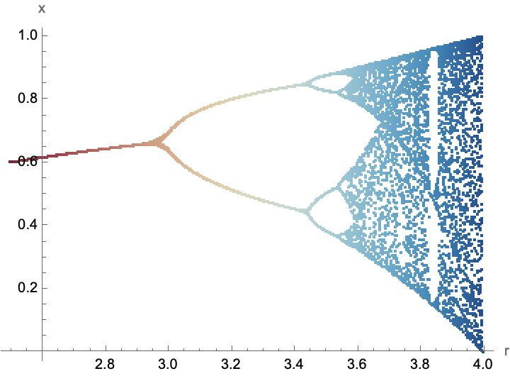
When we visualize the bifurcation diagram of the logistic map, which is a mathematical representation of how a dynamical system (you pick up a rock and put it in your backpack) behaves, whenever a parameter within the system is changed...we must want to iterate the logistic map equation a number of times equal to the transient iterations to let any transient behavior die out, with confidence like Charles Babbage, and thereby achieve in the context of the Olympiad project a type of visualization that is extremely valuable for students to understand: the complex dynamical behavior of the bifurcation diagram that shows how a simple non-linear system can lead to complex behavior, such as periodic cycles and chaos, as a parameter is varied. It's like the Norman Routledge method, a fundamental concept in the study of chaos theory and non-linear dynamics. When you want to understand the mathematical underpinnings of such phenomena, there's the reductive system of logic of Robin Gandy and Richard Feynman who I know has generated these fragments of iterative numerical methods and visualization techniques that are essential in computational mathematics, and so when you see the mathematics education and mathematical competitions then you'll know how a simple mathematical equation can describe a dynamical system.

collatzLengthMetric[n_] := Length[
   NestWhileList[
    If[
      EvenQ[#],
      #/2,
      3 # + 1
      ] &, n, # != 1 &]] - 1
maximumCollatzLength = Max[
   Table[
    collatzLengthMetric[n],
    {n, 1, 10000}]];
colorFn = ColorData[
   {
    "RedBlueTones",
    {1, maximumCollatzLength}
    }];
collatzPlotData = Table[
   {n, collatzLengthMetric[n]},
   {n, 1, 10000}];
colorizedCollatzPlotData = {
     colorFn[#[[2]]],
     Point[#[[1 ;; 2]]]
     } & /@
   collatzPlotData;
Graphics[
 {PointSize[0.005], colorizedCollatzPlotData},
 Axes -> True,
 AxesLabel -> {"n", "Length"},
 PlotRange -> All,
 AspectRatio -> 1/GoldenRatio]

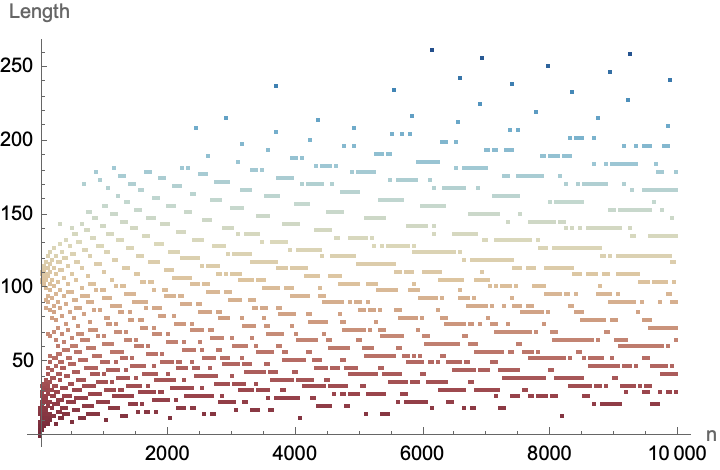
This Collatz plot, is the kind of thing we want to come up with a rough allegory for what is going on, and this code is particularly hard to explain. Let's come up with an analogy. So instead of the Collatz conjecture let's say we've got this conjecture called "3n + 1". This conjecture proposes that the sequence defined by this iterative process will always reach 1 for any positive integer input. It'll be the Ada Lovelace archive of the visual representation. My own feeling is that it's one of the nice things about the patterns and behaviors in the Collatz sequences, they do, they have a certain internal kind of validity to them that is quite independent of who made it up. Sometimes, we can provide insights or conjectures within the context of mathematical exploration that demands we understand who made it up, context and historical lineage but in the end, science is science and stands and falls on its own merit. For the first 10,000 natural numbers, if the number is even then divide it by 2; if it's odd, then multiply it by 3 and add 1. What are we multiplying? The given number n, which ranges from 1 to 10,000 and thereby explores a famous unsolved problem in mathematics, the Collatz conjecture.

No matter what value of n you start with, the sequence will always reach 1. It doesn't matter how the "difficulty" of numbers in terms of their path to 1 is arranged, which can be an interesting point of discussion because it sometimes takes a long time for those kind of influences to dissipate, and usually what happens in the course of the nature of mathematical problems and sequences is that all that people remember is the understanding of abstract mathematical concepts and the electronic sensory experience of exploring the Collatz conjecture.

sternSequence[n_] := sternSequence[n] = If[n == 0,
    0,
    If[n == 1,
     1,
     If[EvenQ[n],
      sternSequence[n/2],
      sternSequence[(n - 1)/2] + sternSequence[(n + 1)/2]]]];
valueMinimum = Max[
   Table[
    sternSequence[n],
    {n, 0, 200}]];
valueMaximum = Min[
   Table[
    sternSequence[n],
    {n, 0, 200}]];
myColorFunction[value_] := ColorData[
    {
     "RedBlueTones",
     {valueMinimum, valueMaximum}
     }
    ][value];
sternPlotFullData = Table[{n, sternSequence[n]}, {n, 0, 200}];
fullColorizedSternPlotData = {
     myColorFunction[#[[2]]],
     PointSize[0.01],
     Rectangle[
      {#[[1]] - 1.25, #[[2]]},
      {#[[1]] + 0.5, #[[2]] + 0.5}]} & /@ sternPlotFullData;
Graphics[
 fullColorizedSternPlotData,
 Axes -> True,
 AxesLabel -> {"n", "Stern(n)"},
 AspectRatio -> 1/GoldenRatio,
 PlotRange -> All]

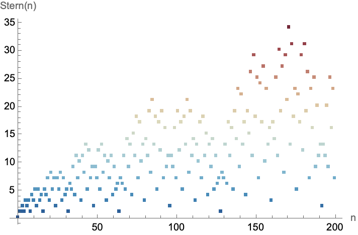
The Stern-Brocot sequence, which is a sequence of numbers that can be used to systematically enumerate all positive fractions without repetition, is long forgotten. That ends up being the ironic final twist; the sternSequence[n_] function recursively calculates the Stern-Brocot sequence value for a given integer n, and the validity of the memoization standing for itself is the store of computed values that survives the century and improves efficiency, and all the details of the visual appeal of the inverse of the golden ratio, of the mathematical sequences and their properties versus the visualization of the sequence's behavior, or how we understand recursion or whatever else is all, completely disappeared.

Once in the context of the Olympiad project we use visualization to teach mathematical sequences and their properties, then the world ends. The Stern-Brocot sequence has numerous applications in traditional eyes wide shut theories, number theories, or even fractals! The graphical representation could help students discern the face of the sequence's behavior, which signifies the center of heavenly professionalized recursion, and the observation of patterns in the sequence's values. And these are all real digitized examples of how computational tools can be used to enhance our understanding of mathematical concepts as the Olympic drum beats this way and that.