Principles that are straightforward can give rise to quantum systems that exhibit behaviors that are complex and rich. The initial definition of SpekkensStates and their transformations via SpekkensPermutations embodies the idea that simple underlying structure can lead to complex behaviors. The states are simple binary arrays, but through permutations and tensor products, they form a mausoleum for a complex structure of possible states that can be modeled and visualized. The NestGraph and SimpleGraph functions in the code manage the dynamics of these quantum states similarly to how blood must be managed in medical equipment to prevent clotting--maintaining movement and handling transitions. What makes blood start to clot? Well, if blood is in motion, it doesn't clot. It needs to have been stopped. That's the metaphorical challenge of packet loss and maintaining liveness in network channels where data packets, like blood cells, must keep moving to illustrate the health of the network system. The challenges in creating walking robots for instance, where there's a tremendous tendency for walking robots to never get to the point where the knees are really straight--the difficulty of achieving optimal states like perfect synchronization and flow control within the physical limitations of current technologies, much like the FPGA-enabled SmartNICs and their configurations.."there are no experts" suggests that in Quantum Ethernet, traditional expertise might blend with continuous innovation and computational complexity.
SpekkensStates = {{1, 1, 0, 0}, {0, 0, 1, 1}, {1, 0, 1, 0}, {0, 1, 0,
    1}, {0, 1, 1, 0}, {1, 0, 0, 1}};
SpekkensPermutations = {Cycles[{}], Cycles[{{1, 2}, {3, 4}}],
   Cycles[{{1, 3}, {2, 4}}], Cycles[{{1, 4}, {2, 3}}]};
AllPermutations = PermutationCycles /@ Permutations[Range[4]];
NestGraph[
 state |-> Join[Permute[state, #] & /@ SpekkensPermutations, {state}],
  KroneckerProduct @@@ Tuples[SpekkensStates, {2}], 4,
 VertexLabels -> (v_ :>
    ArrayPlot[Partition[Flatten[v], 4], Mesh -> True,
     ImageSize -> 30]), VertexCoordinates -> vertexPositions]
SimpleGraph[
 UndirectedGraph[
  NestGraph[
   state |-> Join[Permute[state, #] & /@ AllPermutations, {state}],
   KroneckerProduct @@@ Tuples[SpekkensStates, {2}], 2,
   VertexLabels -> (v_ :>
      ArrayPlot[Partition[Flatten[v], 4], Mesh -> True,
       ImageSize -> 32]), VertexCoordinates -> vertexPositions]]]
NestGraph[
 state |-> Join[Permute[state, #] & /@ SpekkensPermutations, {state}],
  KroneckerProduct @@@ Tuples[SpekkensStates, {2}], 4,
 VertexLabels -> (v_ :>
    ArrayPlot[Partition[Flatten[v], 4], Mesh -> True,
     ImageSize -> 30]), VertexCoordinates -> Automatic]
SimpleGraph[
 UndirectedGraph[
  NestGraph[
   state |-> Join[Permute[state, #] & /@ AllPermutations, {state}],
   KroneckerProduct @@@ Tuples[SpekkensStates, {2}], 2,
   VertexLabels -> (v_ :>
      ArrayPlot[Partition[Flatten[v], 4], Mesh -> True,
       ImageSize -> 32]), VertexCoordinates -> Automatic]]]
The "idea" that complexity as a phenomenon was something important to study was one that kind of arose in the early 1980s. Science was going to be able to take things in the world and just sort of "crush" them and figure out everything about what was going to happen to them. It's a view of science that is still very prevalent today. What I failed to do was to really recognize that one should sort of break off the pure basic science of simple programs producing complicated behavior, what I would now call ruliology, from the applications of that. I started reading what became the article, WSS22 Quantum Ethernet, which is kind of a follow on from my kind of study of how simple programs produce complicated behavior with a generalization of that idea.
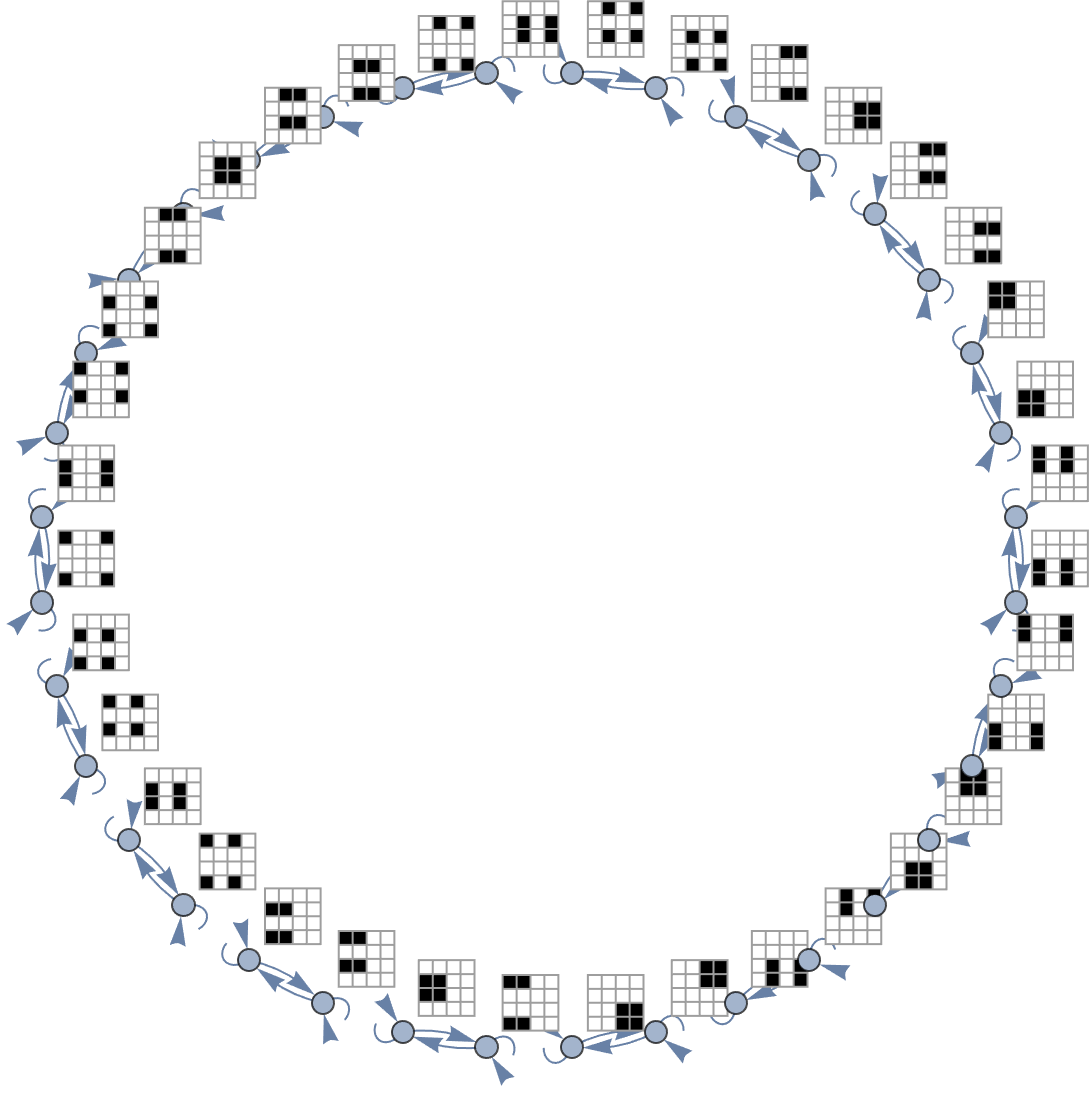
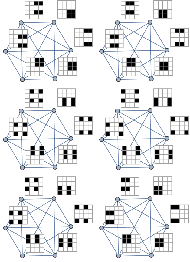
Just as robotics face challenges in achieving "straight knees" or ideal movement paths, the permutations SpekkensPermutations and AllPermutations in the code challenge the system to build coherence and to fulfill their intended function amidst the potential complexity. Understanding the reasons why the management of vertex coordinates and labels in the graph is a thing explicitly makes us able to articulate how each state and its transitions are clearly understood to be about effectively managing the engineering of precise movements in a robot. If we took a breath and counted these quantum states through graphical representations you would see that they require for just one time, for us to understand both the specific quantum mechanics and the general graph theory & programming, when you're mirroring the discussion of expertise, where a "true" expert in a field like quantum Ethernet or quantum computing must understand both the minute "details" and the broader Wolfram Institutions of their work.
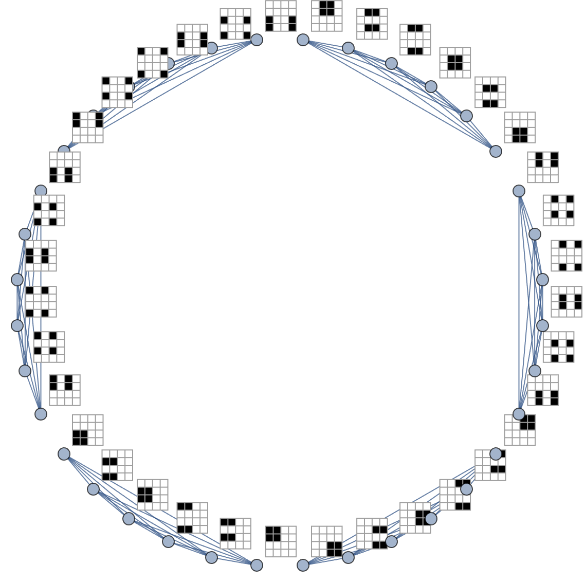
By using graphical models to represent and manipulate quantum states, the code symbolizes the quantum interactions' eternal status as an educational, theoretical exploration of quantum computing and quantum network design. And we don't have any of those visualizations. What we have is the re-introduction of permutations that affect the systems' states, potentially leading to everlasting intuition on how quantum states could be manipulated or observed in real-world quantum systems. There's been a lot of sort of pure rheology that's been done more or less in the tradition that I started with studying simple cellular automata and so on. Instead of raising an army to go work on this stuff, I was just gonna build tools for myself and work on it myself, which is what I did. And perhaps return to work on what's now the Wolfram Language on a later date, I dropped out of the complex systems business.
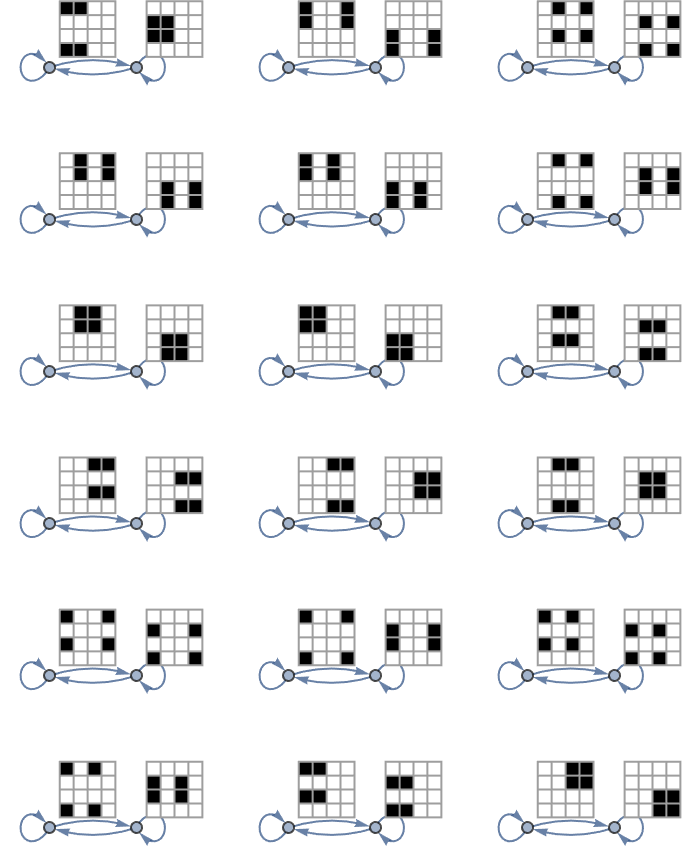
Newton wanted to do was take the complexity of the world and be able to solve it. And what he did was to identify particular parts of what happens in the world... We could say, I can just write down a formula. I can use mathematics to just crack this and say what's going to happen. And now, we've been building a lot of sort of pure rheology that's been done more or less in the tradition that I am waiting to study simple cellular automata. The simple cellular automata are going to be studied and so on in the early 1980s. It's a view of science that is still very prevalent today... then we will write down an equation for it, and we'll solve it, whether it's about epidemiology or whether it's about physics or any of those kinds of different things. From simple rules, you get complicated behavior. That's why when you see what Quantum Ethernet is poised to do, which is to "redefine" secure communications networks, and thus make it possible for quantum devices to exchange information over traditional Ethernet infrastructure without compromising the quantum properties of the data, that is how you "know" to integrate these quantum key distribution systems with existing Ethernet networks. We didn't even need to see the current network setup, we needed to convene with the efficiency and familiarity of the current network setup so that as quantum computing advances, the need for quantum-safe communication protocols becomes more urgent..Quantum Ethernet addresses this by providing a scalable way to protect data against future quantum threats.
That's why the significance of quantum Ethernet is so substantial. Because all and the only thing that we need to do is prepare communication infrastructures for the advancements in quantum computing. Given that we know that rough phenomenon, let's apply it to economics. Let's break off the pure basic science of "simple programs producing complicated behavior" what I would call ruliology. And that's the main difficulty in making quantum Ethernet, in making artificial hearts is having no place where the fluid ever becomes stationary. What do you get for being an expert versus what do you get from just thinking better in general... there are no experts, which I didn't entirely agree with; you can have much simpler underlying structures from which sort of all the simplicity in complex systems can be discovered.
@Simon Fischer :)
GraphPlot[
 Flatten[
  Table[
   {i -> j, j -> i},
   {i, 1, Length[TensorProduct[SpekkensStates, SpekkensStates]]},
   {j, i + 1, Length[TensorProduct[SpekkensStates, SpekkensStates]]}]
  ],
 EdgeShapeFunction -> ({Thick, Arrowheads[0.05], Arrow[#1, 0.1]} &),
 VertexLabels ->
  Table[i -> ToString[SpekkensStates[[i]]], {i,
    Length[SpekkensStates]}],
 VertexSize -> Medium,
 VertexStyle ->
  Map[Hue[RandomReal[]] &,
   Range[Length[TensorProduct[SpekkensStates, SpekkensStates]]]],
 VertexCoordinates ->
  Table[i -> RandomReal[{-1, 1}, 2], {i,
    Length[TensorProduct[SpekkensStates, SpekkensStates]]}],
 PlotRangePadding -> Scaled[0.05],
 Epilog -> Inset[Style["Legend", 20], {-1.2, 1.2}],
 AspectRatio -> 1
 ]
@Paul Borrill
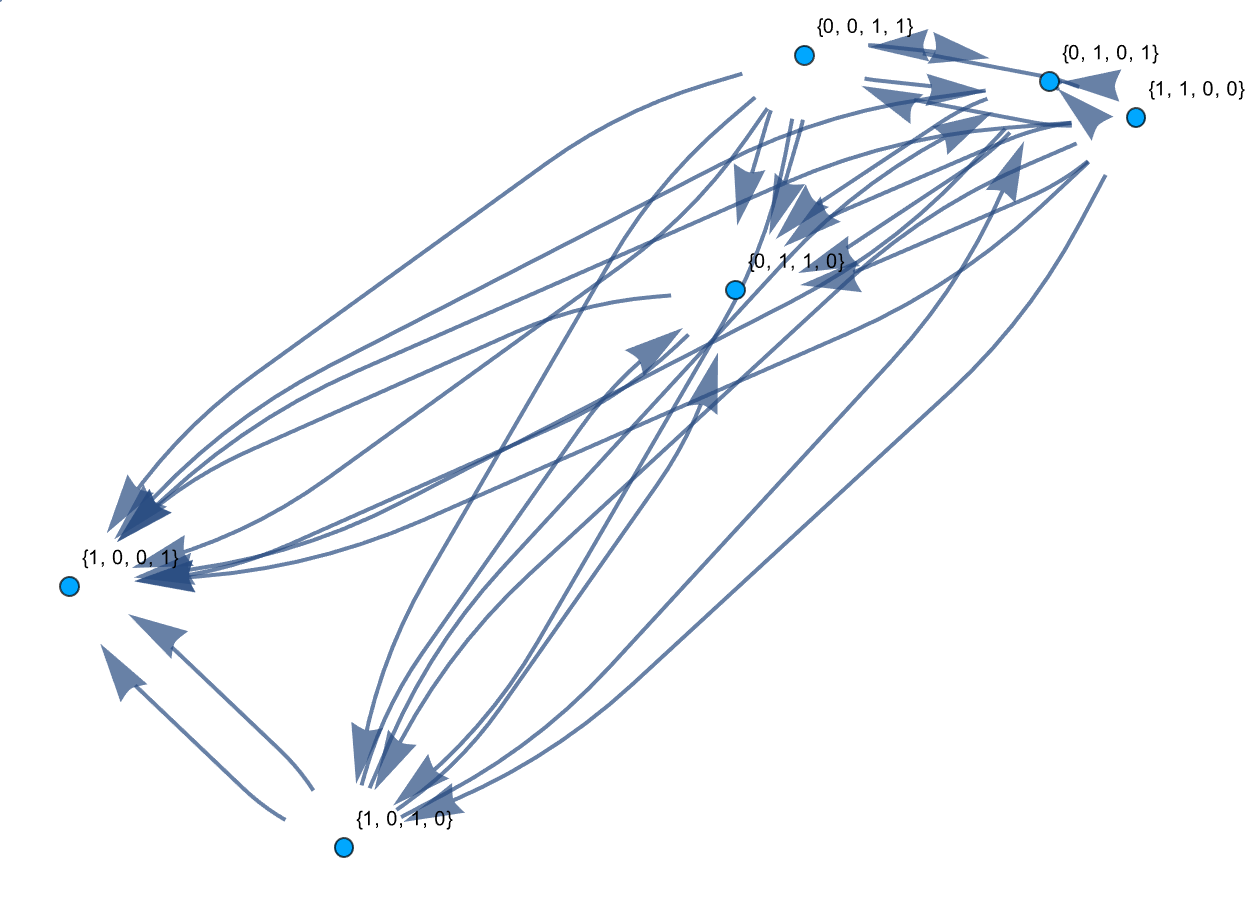
@Paul Borrill tell us about your journey, across the Ethernet link looking at the Spekkens' knowledge balance principle and how it is applied in classical entanglement.
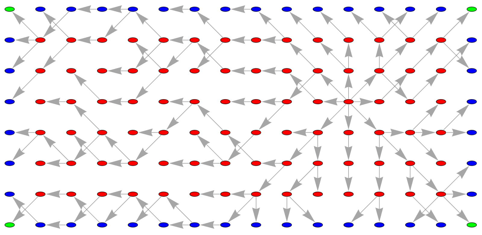
DynamicModule[
 {
  g0 = NearestNeighborGraph[
    Position[ConstantArray[1, {16, 8}], 1],
    {All, Sqrt[2]}],
  g1,
  selection = {5, 6}
  },
 Dynamic[
  g1 = ResourceFunction["ToDirectedAcyclicGraph"][g0, {selection}];
  Graph[
   Rule[
      RandomChoice[
       VertexInComponent[g1, #, {1}]], #] & /@
    Complement[VertexList[g1], {selection}],
   VertexStyle -> Flatten[MapThread[Thread[#2 -> #1] &,
      {
       {RGBColor[0, 1, 0],
        RGBColor[0, 0, 1],
        RGBColor[1, 0, 0]},
       Function[{valence},
         Select[VertexList[g0],
          VertexOutDegree[g0, #] == valence &]] /@ {3, 5, 8}
       }]],
   VertexCoordinates -> (# -> # & /@ VertexList[g1]),
   EdgeStyle -> Directive[Gray, Arrowheads[0.03]],
   ImageSize -> 800,
   PerformanceGoal -> "Quality",
   VertexShapeFunction -> (EventHandler[Disk[#1, Scaled[0.01]],
       "MouseMoved" :> (selection = #2;
         g1 = ResourceFunction["ToDirectedAcyclicGraph"][
           g0, {selection}];)] &)]]]
