Hi @Mishal Harish Moideen this is our machine learning fair for feature extraction and classification, I hope we can classify photographs based on their creation date.
nT = NetTake[
   NetModel["ResNet-50 Trained on ImageNet Competition Data"],
   "flatten_0"];
csvTrainData =
  Import["/Users/deangladish/Downloads/10.22000-43/data/dataset/meta.\
csv", "CSV"];
trainDataSample = RandomSample[
   AssociationThread[csvTrainData[[1]] -> #] & /@ Rest[csvTrainData],
   30];
processImages =
  Quiet[Check[ImageResize[Import[#], {224, 224}], Missing[],
      ImageResize::imgio] & /@ trainDataSample[[All, "url"]]];
indicesExists = Position[processImages, _Image] // Flatten;
processImages = processImages[[indicesExists]];
labels = trainDataSample[[indicesExists, "GT"]];
features = nT[processImages];
trainData = Thread[features -> labels];
nn1 = NetChain[
   {LinearLayer[2048],
    BatchNormalizationLayer[],
    ElementwiseLayer[Ramp],
    LinearLayer[70],
    SoftmaxLayer[]},
   "Input" -> Length[First[features]],
   "Output" -> NetDecoder[{"Class", Range[1930, 1999]}]
   ];
dnn1 = NetTrain[
  NetInitialize[nn1],
  trainData,
  "BatchSize" -> 1,
  "MaxTrainingRounds" -> 5
  ]
The model makes me want to use Graph3D to separate different evaluation paths in 3D space.


@Mishal Harish Moideen, I couldn't have put it better, the visualization of the features that contribute to the data classification is larger than life; the intrigue of amassing these insights into the model's inference texture.
csvTestData = csvTrainData;
testDataSample = RandomSample[
   AssociationThread[csvTestData[[1]] -> #] & /@ Rest[csvTestData],
   30];
processTestImages =
  Quiet[Check[ImageResize[Import[#], {224, 224}], Missing[],
      ImageResize::imgio] & /@ testDataSample[[All, "url"]]];
indicesExists = Position[processTestImages, _Image] // Flatten;
testLabels = testDataSample[[indicesExists, "GT"]]
processTestImages = processTestImages[[indicesExists]];
predictions = dnn1[nT[processTestImages]]
Thank you, @Mishal Harish Moideen . The working fluid is not electrons in electronics but there are actual processes that go on that we can think of as computations just as what happens in molecular biology. One day, people will be surprised that there was a time that the world wasn't made of computers.


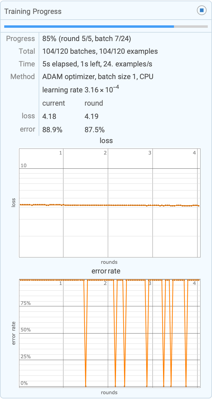
That was the best feature extraction process that I have ever had in my entire life, the very first model we train using the training dataset with the loss function and error rate monitor creates an enriching and memorable balance of objects in each year for improved accuracy like the city of neural nets, it creates an atmosphere of mystique when you mask the gradient over the original image, providing an intuitive inference of the features that lead to a specific year classification.
correctPredictions =
  Total@MapThread[Boole[#1 == #2] &, {predictions, testLabels}];
accuracy = correctPredictions/Length[predictions];
highestFrequency = Commonest[testLabels][[1]];
accuracyBaseline =
  Count[testLabels, highestFrequency]/Length[testLabels];
singleEvaluationTime =
  First@AbsoluteTiming[dnn1[nT[First[processTestImages]]]];
batchTimeProcessImages =
  First@AbsoluteTiming[dnn1[nT[processTestImages]]];
evaluationSpeedProcessImages =
  Length[processTestImages]/batchTimeProcessImages;
numberOfTestExamples = Length[testLabels];
accuracy =
  Total@MapThread[Boole[#1 == #2] &, {predictions, testLabels}]/
   numberOfTestExamples;
highestFrequency = Commonest[testLabels][[1]];
accuracyBaseline =
  Count[testLabels, highestFrequency]/numberOfTestExamples;
cm = ClassifierMeasurements[dnn1, nT[processTestImages] -> testLabels];
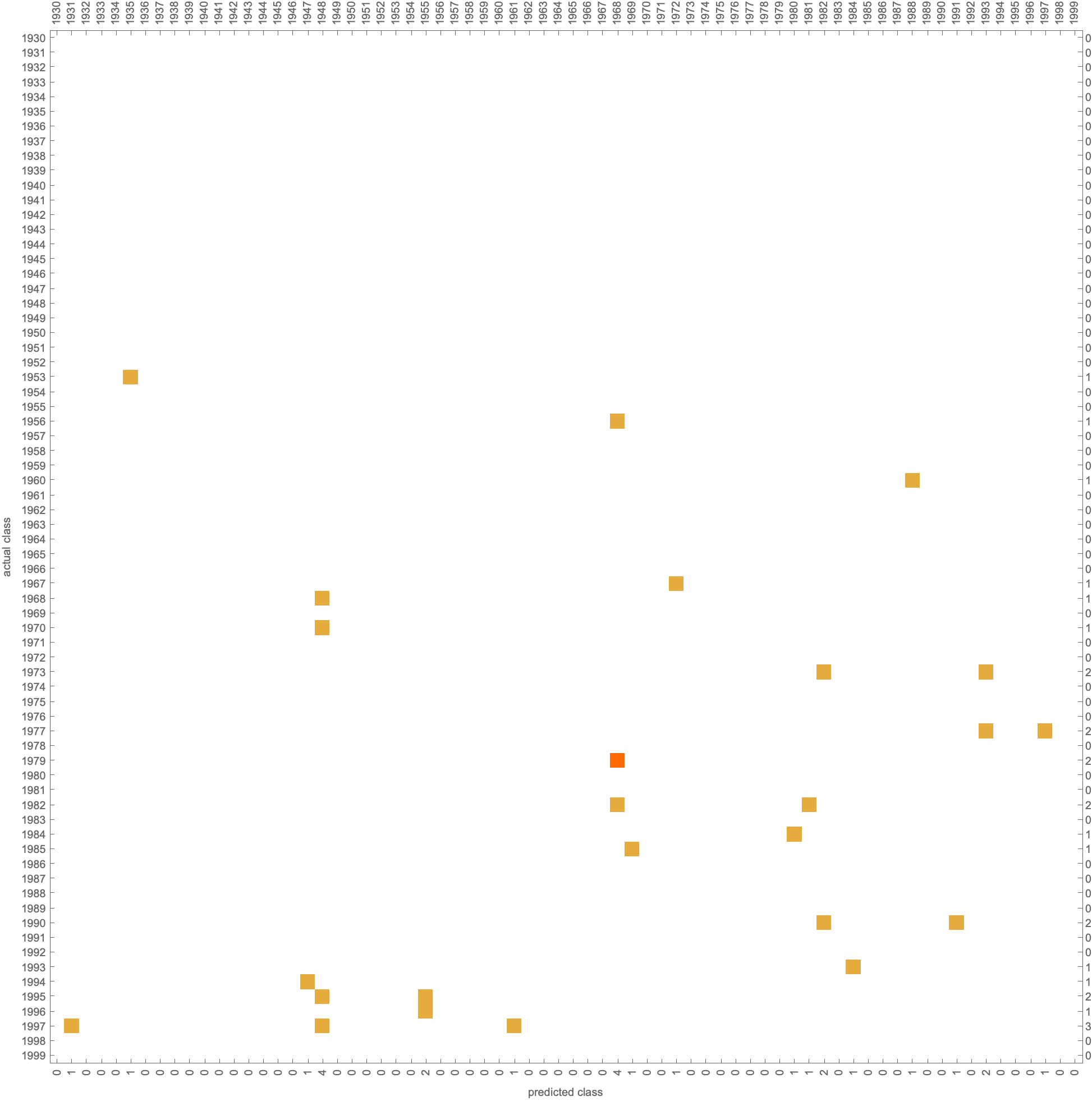
cm["ConfusionMatrixPlot"]
roc = cm["ROCCurve"];
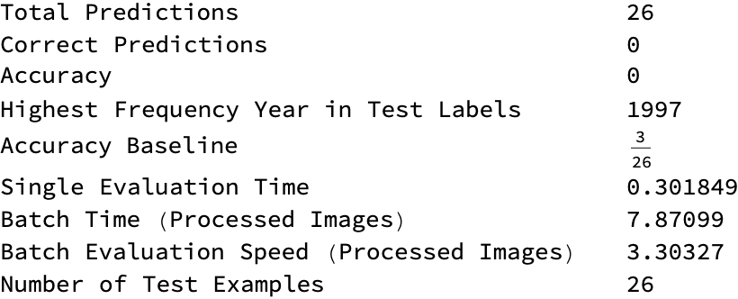
statistics = {{"Total Predictions", Length[predictions]},
   {"Correct Predictions", correctPredictions},
   {"Accuracy", accuracy},
   {"Highest Frequency Year in Test Labels", highestFrequency},
   {"Accuracy Baseline", accuracyBaseline},
   {"Single Evaluation Time", singleEvaluationTime},
   {"Batch Time (Processed Images)", batchTimeProcessImages},
   {"Batch Evaluation Speed (Processed Images)",
    evaluationSpeedProcessImages},
   {"Number of Test Examples", numberOfTestExamples}};
table = TableForm[statistics]
confusionMatrixPlot =
  ArrayPlot[cm["ConfusionMatrix"], FrameTicks -> {True, True},
   ColorFunction -> "TemperatureMap", PlotLabel -> "Confusion Matrix"];
predictionsBarChart =
  BarChart[BinCounts[predictions], ChartLabels -> Automatic,
   PlotLabel -> "Distribution of Predictions"];
evaluationTimes =
  Map[First@AbsoluteTiming[dnn1[nT[#]]] &, processTestImages];
evaluationTimesHistogram =
  Histogram[evaluationTimes,
   PlotLabel -> "Distribution of Evaluation Times"];
classDistributionPieChart =
  PieChart[Counts[testLabels], ChartLabels -> Automatic,
   PlotLabel -> "Class Distribution in Test Labels"];
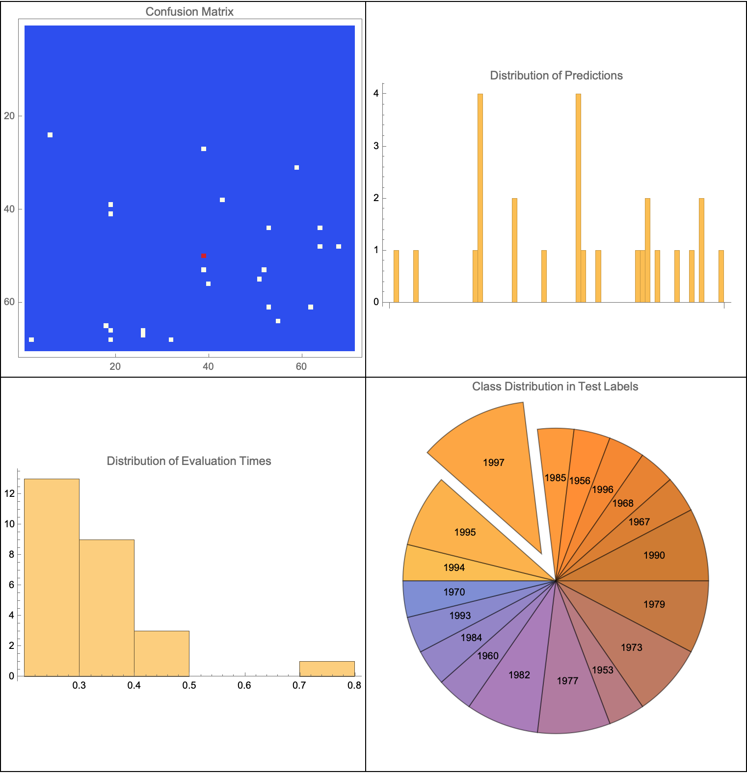
Grid[{{confusionMatrixPlot,
   predictionsBarChart}, {evaluationTimesHistogram,
   classDistributionPieChart}}, Frame -> All]

As you run the neural net it's not learning new stuff.

That's the experience of the single us, one can imagine replacing it; how this relates to the things we already know or how a significant number of predictions are made close to the actual year; it's like how the GOTO combinator implementation in C++ can be converted into an if statement and then the part of GOTO will be in one of the true/false blocks @Mishal Harish Moideen , with unconditional JMP in assembly level, so it can be handled.

What a world! Having an equal number of photographs for each year to avoid bias..maybe there is some incredibly clever way to do cancer immunotherapy but to get there involves this radical change..to get there, in incremental steps. It's only by going far out, and that's a sort of difficult thing to reach by this incremental approach, the bundle of threads that is branching and merging. I'm seeing the pop-up called "Training Progress" that disappears right away.