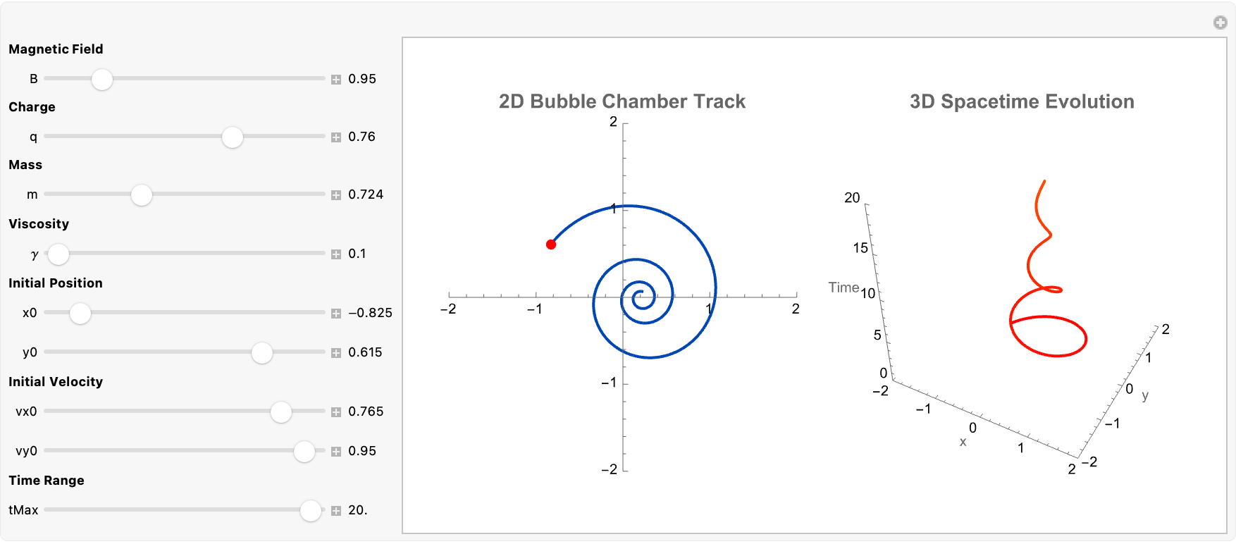
The differential equations for setting up particle trajectories, we can look at physical effects and computational methods and offer new avenues for classroom exploration and research. We simulate the spiral trajectories of charged particles in a bubble chamber using differential equations that incorporate the Lorentz force and a viscous drag term. From our size up to the scale of the universe is 26 orders of magnitude, from our size down to the elementary length is a "100" order of magnitude. So there's a lot more room going down than up. You could in principle encode that computational activity in this microscopic stuff more than you could encode it by building a computer that's the size of a galaxy.

Manipulate[
 Module[{eqns, sol, trajectory2D, trajectory3D, 
   color = Hue[0.6, 1, 0.7]}, 
  eqns = {m x''[t] == q B y'[t] - \[Gamma] x'[t], 
    m y''[t] == -q B x'[t] - \[Gamma] y'[t], x[0] == x0, y[0] == y0, 
    x'[0] == vx0, y'[0] == vy0};
  sol = NDSolve[eqns, {x, y}, {t, 0, tMax}];
  trajectory2D = {x[t], y[t]} /. sol[[1]];
  trajectory3D = {x[t], y[t], t} /. sol[[1]];
  GraphicsRow[{ParametricPlot[trajectory2D, {t, 0, tMax}, 
     PlotRange -> {{-2, 2}, {-2, 2}}, PlotStyle -> color, 
     ImageSize -> 300, 
     PlotLabel -> Style["2D Bubble Chamber Track", Bold, 14], 
     Epilog -> {Red, PointSize[0.03], Point[{x0, y0}]}, 
     AspectRatio -> 1], 
    ParametricPlot3D[trajectory3D, {t, 0, tMax}, 
     PlotRange -> {{-2, 2}, {-2, 2}, {0, tMax}}, PlotStyle -> color, 
     ImageSize -> 300, 
     PlotLabel -> Style["3D Spacetime Evolution", Bold, 14], 
     BoxRatios -> {1, 1, 1}, AxesLabel -> {"x", "y", "Time"}, 
     ColorFunction -> (Hue[#3/tMax] &), Boxed -> False, 
     AxesEdge -> {{-1, -1}, {1, -1}, {-1, -1}}]}]], 
 Style["Magnetic Field", Bold], {{B, 1.5}, 0.1, 5, 
  Appearance -> "Labeled"}, 
 Style["Charge", Bold], {{q, -1}, -2, 2, Appearance -> "Labeled"}, 
 Style["Mass", Bold], {{m, 0.5}, 0.1, 2, Appearance -> "Labeled"}, 
 Style["Viscosity", Bold], {{\[Gamma], 0.3}, 0.1, 5, 
  Appearance -> "Labeled"}, 
 Style["Initial Position", Bold], {{x0, 0}, -1, 1, 
  Appearance -> "Labeled"}, {{y0, 0}, -1, 1, Appearance -> "Labeled"},
  Style["Initial Velocity", Bold], {{vx0, 0}, -1, 1, 
  Appearance -> "Labeled"}, {{vy0, 1}, -1, 1, 
  Appearance -> "Labeled"}, 
 Style["Time Range", Bold], {{tMax, 10}, 5, 20, 
  Appearance -> "Labeled"}, ControlPlacement -> Left, 
 SynchronousUpdating -> False, 
 TrackedSymbols :> {B, q, m, \[Gamma], x0, y0, vx0, vy0, tMax}]

Relativistic Particle Acceleration

When particles are accelerated to speeds approaching that of light, you say look at it and it's not at the speed of light. Sure the classical equations of motion "say" it's at the speed of light but it's not. That's when we include relativistic effects; one natural extension (for whom) is to modify the momentum term. In the classical case, momentum is given by p = m v; however, relativistically we get something more like:

m x''[t] == q B y'[t] - γ x'[t]

which roughly translates to:

D[γ[v[t]] m x'[t], t] == q B y'[t] - γ x'[t]

which is "basically" the same thing except it accounts for the time derivative of the relativistic momentum. One might say limitedly incorporating this factor into the differential equations adds a layer of complexity that better represents experimental conditions in high-energy physics. The time derivative modification not only helps in exploring the transition between classical and relativistic regimes but also paves the way for "discussions" on energy-momentum conservation and modern accelerator physics.

Manipulate[
 Module[{eqns, sol, trajectory}, 
  eqns = {m x''[t] == q B y'[t] - \[Gamma] x'[t], 
    m y''[t] == -q B x'[t] - \[Gamma] y'[t], x[0] == x0, y[0] == y0, 
    x'[0] == vx0, y'[0] == vy0};
  sol = NDSolve[eqns, {x, y}, {t, 0, maxtime}];
  trajectory = {x[t], y[t]} /. sol[[1]];
  ParametricPlot[trajectory, {t, 0, maxtime}, 
   PlotRange -> {{-2, 2}, {-2, 2}}, 
   PlotStyle -> Directive[Thick, ColorData["Rainbow"][q]], 
   Epilog -> {{LightBlue, Opacity[0.1], 
      Rectangle[{-2, -2}, {2, 2}]}, {Blue, Arrowheads[0.06], 
      Arrow[{{-1.8, 1.8}, {-1.8 + 0.5 B, 1.8}}], 
      Text[Style["B Field Direction", 10], {-1.3, 1.8}]}, Red, 
     PointSize[0.02], Point[trajectory /. t -> currentTime]}, 
   AxesLabel -> {"x", "y"}, 
   PlotLabel -> 
    Style["Charged Particle Trajectory in Magnetic Field", 14, 
     Bold]]], 
 Style["Simulation Parameters", Bold, 12], {{m, 1, "Mass (kg)"}, 0.1, 
  5, 0.1, Appearance -> "Labeled"}, {{q, 1, "Charge (C)"}, -2, 2, 0.1,
   Appearance -> "Labeled"}, {{B, 1, "Magnetic Field (T)"}, 0, 5, 0.1,
   Appearance -> "Labeled"}, {{\[Gamma], 0.1, "Viscosity (Ns/m)"}, 0, 
  2, 0.1, Appearance -> "Labeled"}, 
 Style["Initial Conditions", Bold, 
  12], {{x0, 0, "Initial X Position (m)"}, -1, 1, 0.1, 
  Appearance -> "Labeled"}, {{y0, 0, "Initial Y Position (m)"}, -1, 1,
   0.1, Appearance -> "Labeled"}, {{vx0, 1, 
   "Initial X Velocity (m/s)"}, -2, 2, 0.1, 
  Appearance -> "Labeled"}, {{vy0, 0, "Initial Y Velocity (m/s)"}, -2,
   2, 0.1, Appearance -> "Labeled"}, 
 Style["Time Controls", Bold, 
  12], {{maxtime, 10, "Simulation Time (s)"}, 1, 50, 1, 
  Appearance -> "Labeled"}, {{currentTime, 0, "Current Time (s)"}, 0, 
  maxtime, 0.1, Appearance -> "Labeled"}, 
 TrackedSymbols :> {m, q, B, \[Gamma], x0, y0, vx0, vy0, maxtime, 
   currentTime}, ControlPlacement -> Left, 
 SynchronousUpdating -> True, ContinuousAction -> True]

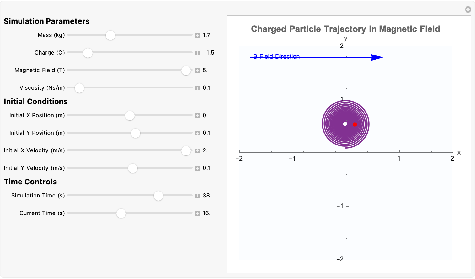
It's the interaction that demonstrates how a charged particle moves in a magnetic field while experiencing viscous drag. When you see the equations of motion that represent Newton's second law applied to the particle in the x and y directions..the first term on the right-hand side of each equation comes from the Lorentz force with the cross-product effects that result in the coupling of x and y derivatives..and the second term represents the viscous drag (damping) force proportional to the velocity. And that's how we know that we have succeeded in defining the simulation as it starts from the initial position (x_0, y_0) and initial velocity (vx0, vy0) state. The particle tracking makes me want to learn how to make visualized solutions. Tracking parameters in the differential equation, how do you show how the spiral changes? Does this remind you of anything? This is exactly and absolutely heartwarming, Syed.

Table[ListLinePlot[NestList[Map[
        Mod[#, 1] &,
        ( {
           {-1.1, 0.9},
           {-1.4, 0.3}
          } ) . #
        ] &, #, i
      ] & /@ {
     {2, 0},
     {0, 1},
     {-3, 0}
     }, PlotStyle -> RGBColor /@
     Permutations[
       Range[3]*137/360,
       3][[-3 ;; -1]],
   PlotMarkers -> {\[SadSmiley], \[NeutralSmiley], \[HappySmiley]},
   MeshFunctions -> {#2 &},
   Mesh -> Automatic,
   MeshStyle -> Opacity[0.1],
   MeshShading -> {Arrowheads[Medium]}] /. 
  Line -> Arrow, {i, 1, 103, 16}]

Now..those interactive spline segments have been such a fun, energetic, and positive journey. Does that remind you of anything? Like Rhodopsin, or purple particles of light.

When it comes down to it the particles sort of kind of start spiraling up, it's amazing. Every once in a blue moon you hear this kind of stuff. Yea, it can be so frustrating making these graphs but as the Earth keeps turning, people's tastes are going to change so what attracts people? Graphics, visuals. People are inspired, they're enthralled by art. Also, where do you see these charge particles of ionized gas occur naturally, Jupiter?

ClearAll["Global`*"];
Manipulate[
 Module[{eqns, sol, trajectory, points, spline, BField}, 
  BField = {0, 0, B};
  eqns = {m x''[t] == 
     q (D[{x[t], y[t], 0}\[Cross]BField, t][[1]]) - \[Gamma] x'[t], 
    m y''[t] == 
     q (D[{x[t], y[t], 0}\[Cross]BField, t][[2]]) - \[Gamma] y'[t], 
    x[0] == x0, y[0] == y0, x'[0] == vx0, y'[0] == vy0};
  sol = NDSolveValue[eqns, {x, y}, {t, 0, tMax}];
  trajectory = 
   ParametricPlot[{sol[[1]][t], sol[[2]][t]}, {t, 0, tMax}, 
    PlotStyle -> Directive[Thick, Blue], 
    PlotRange -> {{-r, r}, {-r, r}}, ImageSize -> 500];
  points = Table[{sol[[1]][t], sol[[2]][t]}, {t, 0, tMax, tMax/100}];
  spline = BSplineFunction[points];
  Show[trajectory, 
   Graphics[{Red, PointSize[0.02], Point[{x0, y0}], Darker@Green, 
     Arrowheads[0.04], 
     Arrow[{{x0, y0}, {x0 + vx0/velocityScale, 
        y0 + vy0/velocityScale}}]}], 
   ParametricPlot[spline[t], {t, 0, 1}, 
    PlotStyle -> Directive[Orange, Dashed]], 
   PlotLabel -> 
    Style["Particle Trajectory with Spline Fit", 14, Bold]]], 
 Style["Particle Properties", Bold, 12], {{m, 1, "Mass"}, 0.1, 5, 0.1,
   Appearance -> "Labeled"}, {{q, 1, "Charge"}, -2, 2, 0.1, 
  Appearance -> "Labeled"}, {{\[Gamma], 0.2, "Viscosity"}, 0, 1, 0.05,
   Appearance -> "Labeled"}, 
 Style["Field Settings", Bold, 12], {{B, 1, "Magnetic Field"}, 0.1, 3,
   0.1, Appearance -> "Labeled"}, {{r, 10, "Plot Range"}, 5, 50, 1, 
  Appearance -> "Labeled"}, 
 Style["Initial Conditions", Bold, 12], {{x0, 0, "x(0)"}, -5, 5, 0.1, 
  Appearance -> "Labeled"}, {{y0, 0, "y(0)"}, -5, 5, 0.1, 
  Appearance -> "Labeled"}, {{vx0, 1, "vx(0)"}, -2, 2, 0.1, 
  Appearance -> "Labeled"}, {{vy0, 1, "vy(0)"}, -2, 2, 0.1, 
  Appearance -> "Labeled"}, {{velocityScale, 2, 
   "Velocity Arrow Scale"}, 1, 5, 0.1, 
  Appearance -> "Labeled"}, {{tMax, 10, "Simulation Time"}, 1, 50, 1, 
  Appearance -> "Labeled"}, 
 TrackedSymbols :> {m, q, \[Gamma], B, x0, y0, vx0, vy0, tMax, r, 
   velocityScale}, ControlPlacement -> Left]

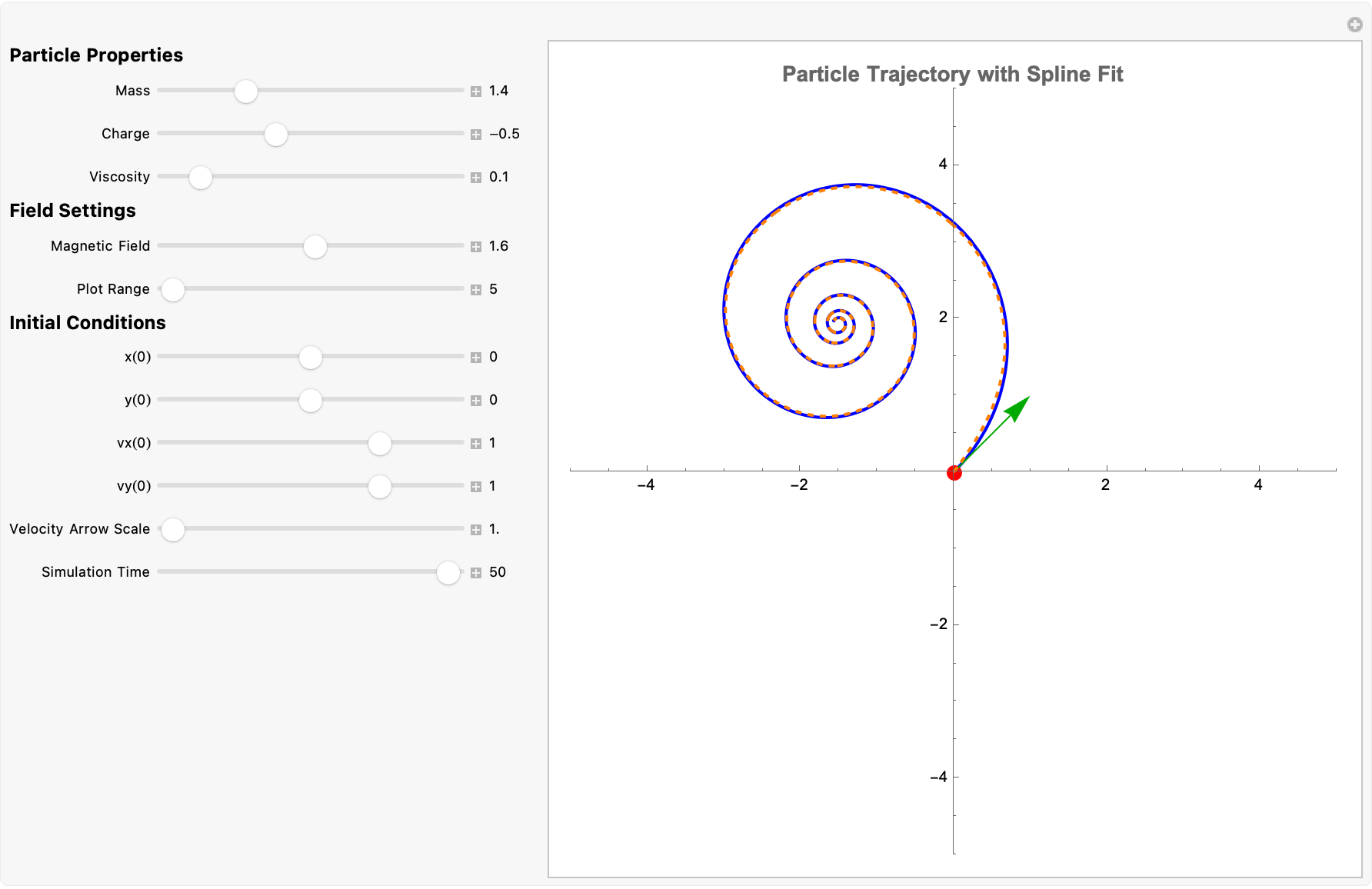
That's when we simulate a charged particle's path in a bubble chamber and then fit a spline, to the computed trajectory. The computer it sort of spans the solar system or the galaxy or whatever. Now one of the things that is the future of physics is that in order to probe length scale you effectively need a lot of energy. Things that are happening at the scale of things inside a proton. The best we can do to probe what's inside a proton, is some kind of bubble chamber. We combine the numerical solution of differential equations with visualization of how the magnetic field is a vector pointing in the z-direction and the scalar B magnetic field strength that is..is set, and the Lorentz Force..on the charged particle, computes the velocity as the time derivative of the position vector {x[t], y[t], 0}. It then forms the cross product with the magnetic field BField and extracts the x- and y- components using [[1]] and [[2]]. That's what the terms −\[Gamma]x'[t] and −\[Gamma]y'[t] are for, they're for modeling the damping due to viscosity in the chamber.

DynamicModule[{m = 1, q = 1, \[Gamma] = 0.1, B = 1, 
  v0 = 1, \[Theta] = 45  °, tmax = 20, sol, vars = {x, y, z}, eqns, 
  plot}, eqns = {m  x''[t] == 
    q  (y'[t]  B - z'[t]  0) - \[Gamma]  x'[t], 
   m  y''[t] == q  (z'[t]  0 - x'[t]  B) - \[Gamma]  y'[t], 
   m  z''[t] == q  (x'[t]  0 - y'[t]  0) - \[Gamma]  z'[t], x[0] == 0,
    y[0] == 0, z[0] == 0, x'[0] == v0  Cos[\[Theta]], y'[0] == 0, 
   z'[0] == v0  Sin[\[Theta]]};
 Manipulate[sol = Quiet@First@NDSolve[eqns, vars, {t, 0, tmax}];
  plot = 
   ParametricPlot3D[Evaluate[{x[t], y[t], z[t]} /. sol], {t, 0, tmax},
     PlotRange -> {{-5, 5}, {-5, 5}, {0, 10}}, 
    ColorFunction -> Function[{x, y, z, t}, Hue[0.7  t/tmax]], 
    PlotStyle -> Thickness[0.005], AxesLabel -> {"X", "Y", "Z"}, 
    BoxRatios -> {1, 1, 1}, ImageSize -> 600, 
    PlotTheme -> "Scientific"];
  Show[plot, 
   Graphics3D[{{Blue, Opacity[0.2], 
      InfinitePlane[{{0, 0, 0}, {1, 0, 0}, {0, 1, 0}}]}, {Red, 
      Arrow[{{0, 0, 0}, {0, 0, 2}}], Text["B Field", {0, 0, 2.2}]}, 
     Sphere[{x[t], y[t], z[t]} /. sol /. t -> tmax, 0.1]}]], {{tmax, 
    20, "Observation Time (s)"}, 1, 50, Appearance -> "Labeled"}, 
  TrackedSymbols :> {tmax}, ControlPlacement -> Left]]

That's probably why the particle tracks numerically solve the 3D differential equations (with the viscous drag) up to the specified tmax and plot how varying physical parameters such as observation time or even mass charge and magnetic field strength, and viscosity affect the trajectory of a charged particle in a magnetic field. The Lorentz force versus the viscous drag, make this a formidable educational tool for studying the bubble chamber-like environment, allowing users to see where the particle is at any moment during the simulation.

DynamicModule[{eqns, soln}, 
 eqns = {m x''[t] == q B y'[t] - \[Gamma] x'[t], 
   m y''[t] == -q B x'[t] - \[Gamma] y'[t], x[0] == 0, y[0] == y0, 
   x'[0] == 0, y'[0] == vy0};
 soln = ParametricNDSolveValue[
   eqns, {x, y}, {t, 0, 10}, {q, B, m, \[Gamma], y0, vy0}];
 Manipulate[
  Module[{xFunc, yFunc, traj, currentPos}, {xFunc, yFunc} = 
    soln[q, B, m, \[Gamma], y0, vy0];
   traj = 
    ParametricPlot[{xFunc[\[Tau]], yFunc[\[Tau]]}, {\[Tau], 0, tmax}, 
     PlotRange -> 3, PlotStyle -> Directive[Red, Thick], 
     AxesLabel -> {"x", "y"}, ImageSize -> 500, 
     GridLines -> Automatic, GridLinesStyle -> LightGray];
   currentPos = {xFunc[tmax], yFunc[tmax]};
   Show[traj, 
    Graphics[{Blue, PointSize[0.03], Point[currentPos], Darker[Blue], 
      Thin, Arrow[{{0, 0}, currentPos}]}], 
    PlotLabel -> 
     Style[StringForm[
       "Particle Trajectory\nCharge: `1`  B: `2`  Mass: `3`\n\
Viscosity: `4`  Time: `5`", q, B, m, \[Gamma], 
       NumberForm[tmax, {3, 1}]], 14, Bold]]], 
  Style["Physical Parameters", Bold, 12], {{q, 1, "Charge (q)"}, -2, 
   2, 0.1, Appearance -> {"Labeled", "Open"}}, {{B, 1, 
    "Magnetic Field (B)"}, 0.1, 5, 0.1, 
   Appearance -> {"Labeled", "Open"}}, {{m, 1, "Mass (m)"}, 0.1, 5, 
   0.1, Appearance -> {"Labeled", "Open"}}, {{\[Gamma], 0.5, 
    "Viscosity (\[Gamma])"}, 0, 2, 0.1, 
   Appearance -> {"Labeled", "Open"}}, 
  Style["Initial Conditions", Bold, 
   12], {{y0, 0.1, "Y Position (y₀)"}, -1, 1, 0.1, 
   Appearance -> {"Labeled", "Open"}}, {{vy0, 1, 
    "Y Velocity (v₀)"}, -2, 2, 0.1, 
   Appearance -> {"Labeled", "Open"}}, 
  Style["Time Control", Bold, 12], {{tmax, 0.1, "Elapsed Time"}, 0.1, 
   10, 0.1, Appearance -> {"Labeled", "Open"}}, 
  ControlPlacement -> Left, 
  TrackedSymbols :> {q, B, m, \[Gamma], y0, vy0, tmax}, 
  Paneled -> True, FrameMargins -> 0]]

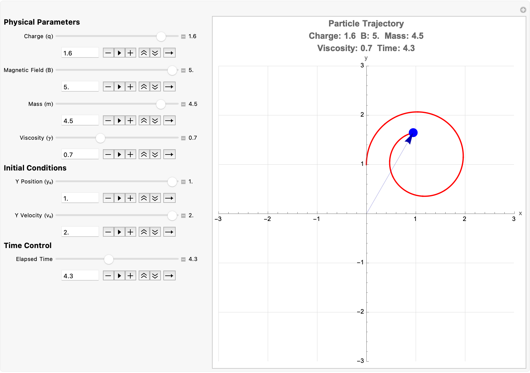
But NAND is functionally complete, but you can represent all these other forms of logic in forms of combinations of NANDS. The subexpressions, the set of differential equations modeling a charged particle's motion in a magnetic field with viscous damping. My physical parameters, use ParametricNDSolveValue to solve these equations, allowing the solution to depend on several physical parameters, initial conditions, and even the elapsed time. And, the visualization of the particle's trajectory in the xy-plane, mark the current position and draw an arrow from the origin, while also tracing the active parameter values. How changes in the physical parameters affect the motion of a charged particle in this bubble chamber environment, and so on and so forth.

Manipulate[
 Module[{eqns, sol, trajectory, dataPoints, splineFit, timeRange = 10,
    radiusData}, 
  eqns = {m x''[t] == q B y'[t] - \[Gamma] x'[t], 
    m y''[t] == -q B x'[t] - \[Gamma] y'[t], x[0] == x0, y[0] == y0, 
    x'[0] == vx0, y'[0] == vy0};
  sol = NDSolve[eqns, {x, y}, {t, 0, timeRange}];
  trajectory = {x[t], y[t]} /. sol[[1]];
  dataPoints = Table[trajectory, {t, 0, timeRange, timeRange/50}];
  splineFit = BSplineFunction[dataPoints];
  radiusData = 
   Table[Norm[trajectory], {t, 0, timeRange, timeRange/100}];
  GraphicsRow[{Show[
     ParametricPlot[trajectory, {t, 0, timeRange}, 
      PlotStyle -> Directive[Blue, Thickness[0.005]], 
      PlotRange -> {{-20, 20}, {-20, 20}}, 
      PlotLabel -> Style["Particle Trajectory", 14, Bold]], 
     ParametricPlot[splineFit[t], {t, 0, 1}, 
      PlotStyle -> Directive[Red, Thickness[0.005], Dashed]], 
     Graphics[{Green, PointSize[Medium], Point[dataPoints]}]], 
    ListLinePlot[radiusData, PlotStyle -> Purple, 
     PlotLabel -> Style["Radius Decay Over Time", 14, Bold], 
     AxesLabel -> {"Time", "Radius"}, GridLines -> Automatic]}, 
   ImageSize -> 800]], 
 Style["Physical Parameters", Bold, 
  12], {{B, 1.5, "Magnetic Field (B)"}, 0.1, 5, 0.1, 
  Appearance -> "Labeled"}, {{q, 1.0, "Charge (q)"}, -2, 2, 0.1, 
  Appearance -> "Labeled"}, {{m, 1.0, "Mass (m)"}, 0.1, 5, 0.1, 
  Appearance -> "Labeled"}, {{\[Gamma], 0.3, "Viscosity (\[Gamma])"}, 
  0, 1, 0.05, Appearance -> "Labeled"}, 
 Style["Initial Conditions", Bold, 12], {{x0, 0, "Initial X"}, -5, 5, 
  0.1, Appearance -> "Labeled"}, {{y0, 0, "Initial Y"}, -5, 5, 0.1, 
  Appearance -> "Labeled"}, {{vx0, 0.5, "Initial Vx"}, -2, 2, 0.1, 
  Appearance -> "Labeled"}, {{vy0, 2.0, "Initial Vy"}, -5, 5, 0.1, 
  Appearance -> "Labeled"}, ControlPlacement -> Left, 
 TrackedSymbols :> {B, q, m, \[Gamma], x0, y0, vx0, vy0}]

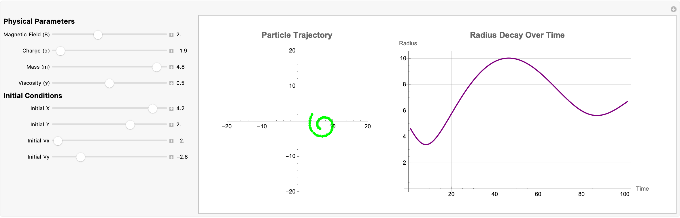
mx′′(t)=qBy′(t)−γx′(t)

my′′(t)=-qBx′(t)−γy′(t)

These two second-order differential equations model the motion of the Lorentz Force wherein qBy'(t) and -qBx'(t) cause the charged particle to curve in the magnetic field. And, the viscous drag terms -γx'(t) and -γy'(t) introduce a damping effect, mimicking energy loss in a viscous medium over a fixed time interval, here set to 10 seconds as stored in the local variable timeRange..the numerical solution for x[t] and y[t] over the interval t ∈ [0, 10]. We sample the "trajectory" at 51 equally spaced time points to create a list of data points along the path, and then compute a BSpline function through these data points, which creates an approximation (red dashed curve) of the trajectory and the radius over time calculation for each time value sampled more finely..the Euclidean norm (distance from the origin) of the trajectory shows how the radius of the particle's path decays or alters over time.

soln = ParametricNDSolveValue[{m x''[t] == q B y'[t] - \[Gamma] x'[t],
     m y''[t] == -q B x'[t] - \[Gamma] y'[t], x[0] == 0, y[0] == y0, 
    x'[0] == 0, y'[0] == vy0}, {x, y}, {t, 0, 20}, {q, B, m, \[Gamma],
     y0, vy0}];
Manipulate[
 Module[{xFunc, yFunc}, {xFunc, yFunc} = 
   soln[qVal, BVal, mVal, \[Gamma]Val, y0Val, vy0Val];
  ParametricPlot[{xFunc[t], yFunc[t]}, {t, 0, tmax}, 
   PlotRange -> {{-10, 10}, {-10, 10}}, AxesLabel -> {"x", "y"}, 
   ImageSize -> 500, 
   PlotLabel -> Style["Charged Particle in Bubble Chamber", Bold, 14],
    Epilog -> {Red, PointSize[0.03], 
     Point[{xFunc[currentT], yFunc[currentT]}]}]], 
 Style["Physical Parameters", Bold], {{qVal, 1, "Charge (q)"}, 0.1, 2,
   Appearance -> "Labeled"}, {{BVal, 1, "Magnetic Field (B)"}, 0.1, 2,
   Appearance -> "Labeled"}, {{mVal, 1, "Mass (m)"}, 0.1, 2, 
  Appearance -> "Labeled"}, {{\[Gamma]Val, 0.1, 
   "Viscosity (\[Gamma])"}, 0, 1, Appearance -> "Labeled"}, 
 Style["Initial Conditions", 
  Bold], {{y0Val, 0, "Initial Y Position"}, -2, 2, 
  Appearance -> "Labeled"}, {{vy0Val, 1, "Initial Y Velocity"}, 0, 2, 
  Appearance -> "Labeled"}, 
 Style["Simulation Controls", Bold], {{tmax, 10, "Trajectory Length"},
   0.1, 20, 
  Appearance -> "Labeled"}, {{currentT, 0, "Animate Particle"}, 0, 
  Dynamic@tmax, AnimationRate -> 1, 
  Appearance -> {"Paused", "Played"}}, ControlPlacement -> Left, 
 TrackedSymbols :> {qVal, BVal, mVal, \[Gamma]Val, y0Val, vy0Val, 
   tmax, currentT}]

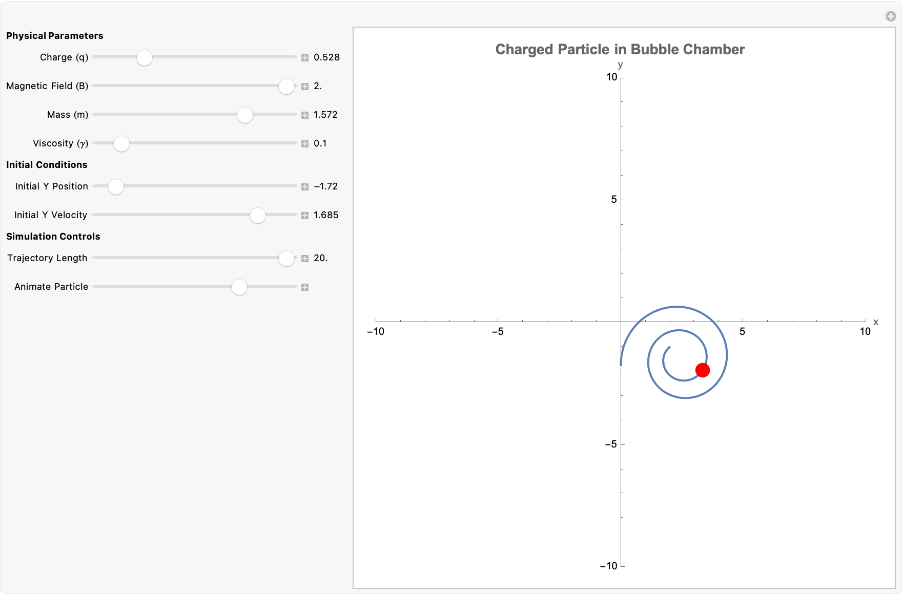
Watch the particle's motion evolve over time, the animation time that allows you to see the particle' location at any moment along the trajectory immediately whenever the differential equations, which include both the Lorentz force and a damping term..let you alter physical parameters such as charge and magnetic field and mass and viscosity..as well as initial y-position and velocity..and the highlight is the current particle position with a red point.