axiomsUMT = {1\[SmallCircle]a_ <-> a, a_\[SmallCircle]1 <-> a};
inits = {1\[SmallCircle]1};
PacletInstall["https://wolfr.am/Multicomputation.paclet",
ForceVersionInstall -> True];
<< Wolfram`Multicomputation`
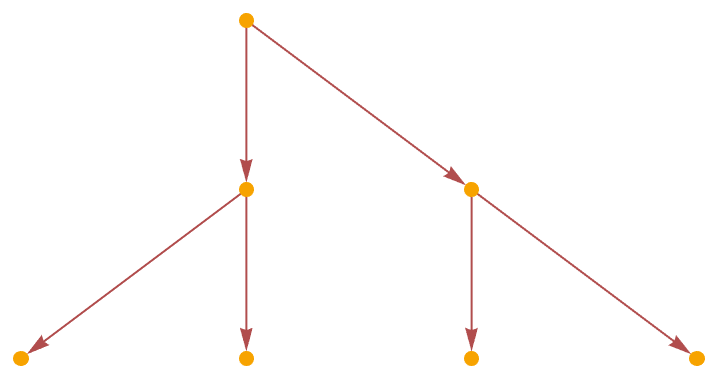
axiomsUMT1 = {1\[SmallCircle]a_ -> a, a_ -> 1\[SmallCircle]a,
a_\[SmallCircle]1 -> a, a_ -> a\[SmallCircle]1};
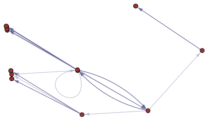
hgm = HypergraphMulti[inits, axiomsUMT1];
graph1 = hgm["Graph",
2,
EdgeStyle -> {_ :>
Directive[Thickness[0.001],
ColorData["FruitPunchColors"][RandomReal[]],
Arrowheads[{{0.01 , 0.7}}], Opacity[0.8]]},
VertexStyle -> {v_ :> ColorData["IslandColors"][RandomReal[]]},
VertexSize -> Large,
VertexShapeFunction -> "Capsule",
GraphLayout -> "SpringElectricalEmbedding",
AspectRatio -> 1/1.5,
ImageSize -> 800
];
graph2 = hgm["Graph",
2,
EdgeStyle ->
Directive[RGBColor[0.3, 0.7, 0.3, 0.7],
Arrowheads[{{0.01 , 0.7}}]],
VertexSize -> Small,
GraphLayout -> "CircularEmbedding",
AspectRatio -> 1/3,
ImageSize -> 800
];
Grid[{{graph1}, {graph2}}]
You, @Aritra Sarkar, have drawn an analogy between video games and the fabric of reality, and I know that the ideas of epistemological limitations and computational resources are new to many.
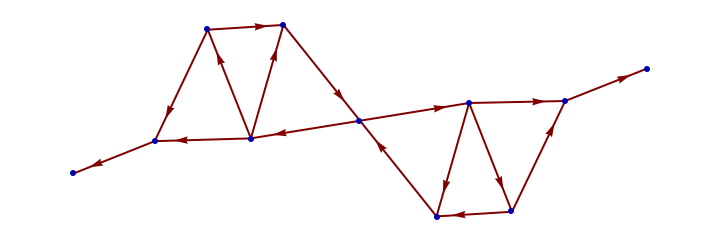
axiomsSGT = {a_\[SmallCircle](b_\[SmallCircle]c_) ->
a\[SmallCircle](b\[SmallCircle]c), (a_\[SmallCircle]b_)\
\[SmallCircle]c_ -> a\[SmallCircle](b\[SmallCircle]c)};
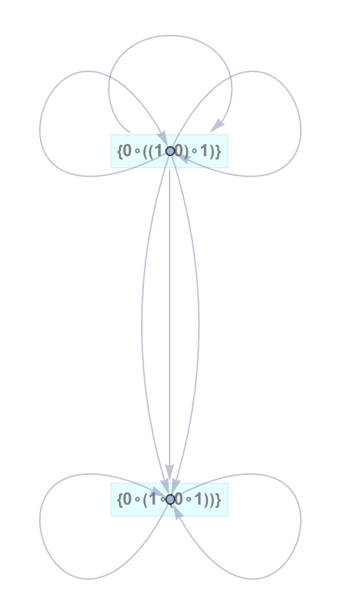
inits = {0\[SmallCircle]((1\[SmallCircle]0)\[SmallCircle]1)};
PacletInstall["https://wolfr.am/Multicomputation.paclet",
ForceVersionInstall -> True];
<< Wolfram`Multicomputation`
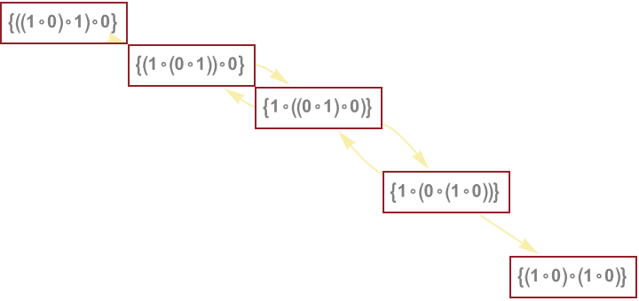
hgm = HypergraphMulti[inits, axiomsSGT];
tree = hgm["Graph", 1,
VertexShapeFunction ->
Function[{pos, v, size},
Inset[Framed[
Style[Wolfram`Multicomputation`FromLinkedHypergraph[v,
"Expression"], Bold, Gray, FontSize -> 12],
FrameStyle -> LightBlue, Background -> LightCyan], pos, size]],
PerformanceGoal -> "Quality",
EdgeStyle -> Directive[RGBColor[0.4, 0.4, 0.6, 0.4]],
GraphLayout -> "LayeredDigraphEmbedding", AspectRatio -> 1/3.5];
hgm2 = hgm["Graph", 2,
EdgeStyle -> Directive[RGBColor[0.4, 0.4, 0.6, 0.4]],
GraphLayout -> "LayeredDigraphEmbedding", AspectRatio -> 1/3];
Show[tree, hgm2]
The observers take in a set of rules.
The observers have a resource limit when we define an observer's proof path.
PacletInstall["https://wolfr.am/Multicomputation.paclet",
ForceVersionInstall -> True];
<< Wolfram`Multicomputation`
axiomsMT1 = {1\[SmallCircle]a_ -> a, a_ -> 1\[SmallCircle]a,
a_\[SmallCircle]1 -> a, a_ -> a\[SmallCircle]1,
a_\[SmallCircle](b_\[SmallCircle]c_) -> (a\[SmallCircle]b)\
\[SmallCircle]c, (a_\[SmallCircle]b_)\[SmallCircle]c_ ->
a\[SmallCircle](b\[SmallCircle]c)};
inits = {1\[SmallCircle]((0\[SmallCircle]1)\[SmallCircle]0)};
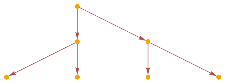
hgm = HypergraphMulti[inits, axiomsMT1];
hgm["Graph", 1,
VertexShapeFunction ->
Function[{pos, v, size},
Inset[Framed[
Style[Wolfram`Multicomputation`FromLinkedHypergraph[v,
"Expression"], Bold, Gray, FontSize -> 12],
FrameStyle -> Directive[Thick, RGBColor[0.2, 0.5, 0.2, 0.2]]],
pos, size]], PerformanceGoal -> "Quality",
EdgeStyle ->
Directive[Thickness[0.001], RGBColor[0.7, 0.2, 0.2, 0.2],
Arrowheads[{{0.01, 0.7}}]], GraphLayout -> "RandomEmbedding",
AspectRatio -> 1/1]
The observers' resource limit defines possible foliations on causal graphs.
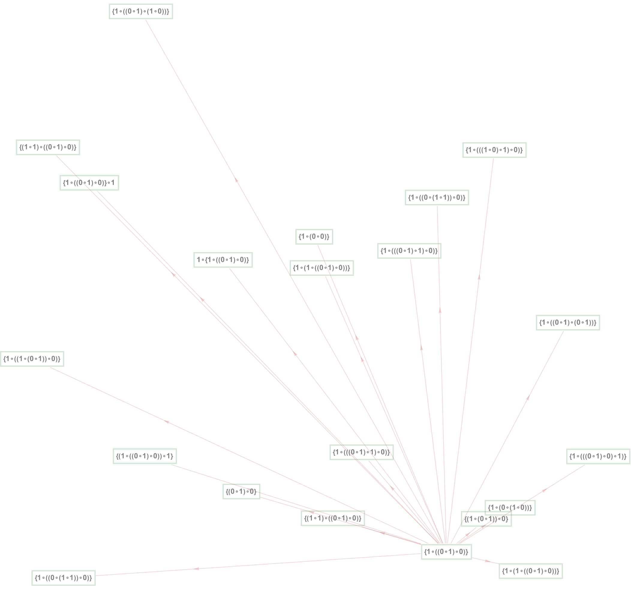
The observers themselves are defined by the standard axiom systems of mathematics.
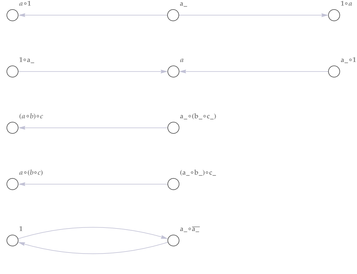
axiomsGT = {1\[SmallCircle]a_ -> a, a_ -> 1\[SmallCircle]a,
   a_\[SmallCircle]1 -> a, a_ -> a\[SmallCircle]1,
   a_\[SmallCircle] (b_\[SmallCircle] c_) -> (a\[SmallCircle]
       b)\[SmallCircle] c, (a_\[SmallCircle] b_)\[SmallCircle] c_ ->
    a\[SmallCircle]( b\[SmallCircle] c), a_\[SmallCircle]
\!\(\*OverscriptBox[\(a_\), \(_\)]\) -> 1, 1 -> a_\[SmallCircle]
\!\(\*OverscriptBox[\(a_\), \(_\)]\)};
edges = axiomsGT /. {x_ <-> y_ :> Rule[x, y]};
Graph[edges, VertexLabels -> "Name", VertexSize -> Medium,
 VertexStyle -> White,
 VertexLabelStyle ->
  Directive[Bold, Gray, FontFamily -> "Palatino", FontSize -> 12],
 EdgeStyle -> RGBColor[0.4, 0.4, 0.6, 0.4], ImageSize -> 600]
The observers are also defined by axioms! The observers take in a set of rules, with a limit of resources, and define proof paths & possible foliations on causal graphs. And they are defined by standard axiom systems of mathematics! @Aritra Sarkar.
axiomLists = {
   {a_\[SmallCircle](b_\[SmallCircle]c_) -> (a\[SmallCircle]b)\
\[SmallCircle]c, (a_\[SmallCircle]b_)\[SmallCircle]c_ ->
     a\[SmallCircle](b\[SmallCircle]c), 1\[SmallCircle]a_ -> a,
    a_ -> 1\[SmallCircle]a, a_\[SmallCircle]1 -> a,
    a_ -> a\[SmallCircle]1},
   {0\[SmallCircle]0 -> 1, 0\[SmallCircle]1 -> 1,
    1\[SmallCircle]0 -> 1, 1\[SmallCircle]1 -> 0},
   {a\[SmallCircle]a -> 1, 0\[SmallCircle]1 -> 1,
    1\[SmallCircle]0 -> 1}
   };
Column[
 Grid[
    Partition[
     ResourceFunction["UnformalizeSymbols"][#], 2],
    Sequence @@ {
      ItemStyle -> {Bold, Gray, FontFamily -> "Palatino",
        FontSize -> 12},
      Spacings -> 1,
      ItemSize -> {13, 2}
      }] & /@ axiomLists]
We finally made it, this is the axiom list I've been waiting for. I can't believe these axiom systems.
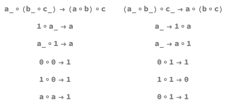
But now that I take a closer look at the punctuation, of the set of rules that defines the proof paths for the initial conditions..this completes the Ruliad!
PacletInstall["https://wolfr.am/Multicomputation.paclet",
  ForceVersionInstall -> True];
<< Wolfram`Multicomputation`
axioms = {a_ -> a\[SmallCircle]a,
   a_\[SmallCircle](b_\[SmallCircle]c_) -> (a\[SmallCircle]b)\
\[SmallCircle](a\[SmallCircle]c), a_\[SmallCircle]a_ -> 0,
   a_\[SmallCircle]0 -> a, (a_\[SmallCircle]b_)\[SmallCircle]c_ ->
    a\[SmallCircle]c, (a_\[SmallCircle]b_)\[SmallCircle]b_\
\[SmallCircle]d_ -> a\[SmallCircle]d};
inits = {1\[SmallCircle]((0\[SmallCircle]1)\[SmallCircle]0)\
\[SmallCircle]1};
trots = 1;
hgm = HypergraphMulti[inits, axioms];
hgm["Graph", trots,
 VertexShapeFunction ->
  Function[{pos, v, size},
   Inset[Framed[
     Style[Wolfram`Multicomputation`FromLinkedHypergraph[v,
       "Expression"], Bold, Gray],
     FrameStyle -> RGBColor[0.678, 0.847, 0.902]], pos, size]],
 PerformanceGoal -> "Speed", EdgeShapeFunction -> None,
 GraphLayout -> "StarEmbedding", ImageSize -> 600]
I'm sorry for the StarEmbedding but yeah this is truly breath-taking and awe-inspiring.
An observer could entail the full Ruliad and just explore the limited subset. And then comes this inundation of the graphs to depict the order of node traversal, with which we can understand the dynamics of the Ruliad and how it can be explored with limited computational resources.
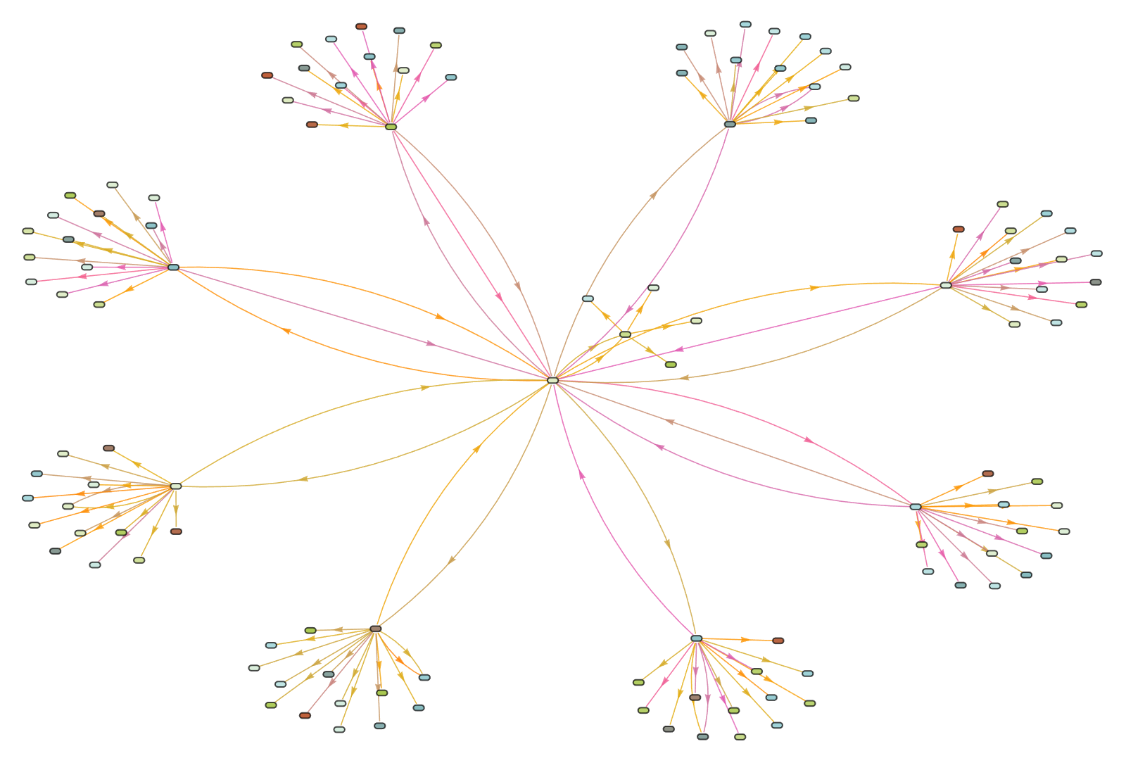
PacletInstall["https://wolfr.am/Multicomputation.paclet",
  ForceVersionInstall -> True];
<< Wolfram`Multicomputation`
axioms = {
   a_\[SmallCircle]a_^-1 -> 1,
   a_^-1\[SmallCircle]a_ -> 1,
   a_\[SmallCircle]1 -> a,
   1\[SmallCircle]a_ -> a,
   a_\[SmallCircle](a_^-1) -> 1,
   (a_^-1)\[SmallCircle]a_ -> 1,
   (a_\[SmallCircle]b_\[SmallCircle]c_) ->
    a\[SmallCircle](b\[SmallCircle]c),
   (a_\[SmallCircle]b_)\[SmallCircle]c_ ->
    a\[SmallCircle](b\[SmallCircle]c),
   a_\[SmallCircle]b_ -> b\[SmallCircle]a,
   a_\[SmallCircle](b_\[SmallCircle]a_^-1) -> b\[SmallCircle]a^-1,
   (a_^-1)\[SmallCircle](b_\[SmallCircle]a_) -> b\[SmallCircle]a,
   (a_\[SmallCircle]b_)\[SmallCircle]b_\[SmallCircle]c_ ->
    a\[SmallCircle]c,
   (a_\[SmallCircle]b_\[SmallCircle]c_)\[SmallCircle]c_\[SmallCircle]\
d_ -> a\[SmallCircle](b\[SmallCircle]d)
   };
inits = {1\[SmallCircle]((0\[SmallCircle]1)\[SmallCircle]0),
   a\[SmallCircle]a^-1, a^-1\[SmallCircle]a};
trots = 2;
hgm = HypergraphMulti[inits, axioms];
I want to show the intricate interconnections within the computational entailment fabric.
g = hgm[
   "Graph",
   trots,
   GraphLayout -> {"SpectralEmbedding", "Rotation" -> 1},
   VertexStyle -> RGBColor[0.88, 0.93, 0.96]
   ];
Show[GraphPlot[g]]
@Aritra Sarkar Yeah! I'm so looking forward to the monoid theory axioms in your color scheme and writing style, please, I know this just seems a little far-fetched but if there's one thing I want to see more of it's the monoid theory axioms.
This is the entailment fabric that induces an ordering on the set of expressions. How would you characterize them? This really breaks down combinatorial logic to NAND and then to SK.
PacletInstall["https://wolfr.am/Multicomputation.paclet",
  ForceVersionInstall -> True];
<< Wolfram`Multicomputation`
axioms = {a_\[SmallCircle] (b_\[SmallCircle] c_) -> (a\[SmallCircle]
       b)\[SmallCircle] c, (a_\[SmallCircle] b_)\[SmallCircle] c_ ->
    a\[SmallCircle]( b\[SmallCircle] c), 1\[SmallCircle]a_ -> a,
   a_ -> 1\[SmallCircle]a, a_\[SmallCircle]1 -> a,
   a_ -> a\[SmallCircle]1};
inits = {1\[SmallCircle]((0\[SmallCircle]1)\[SmallCircle]0)};
trots = 2;
hgm = HypergraphMulti[inits, axioms];
hgm[
 "Graph",
 trots,
 EdgeStyle -> Directive[Thickness[0.01], RGBColor[0.4, 0.4, 0.6, 0.4]],
 GraphLayout -> "RadialEmbedding",
 VertexStyle -> RGBColor[0.2, 0.8, 0.2],
 VertexShapeFunction -> "Star",
 EdgeShapeFunction -> GraphElementData["CurvedArc"]
 ]
It could be interesting to effectively represent the Boolean NAND and XOR operations, maybe create graphs that demonstrate a systematic navigation of the nodes, in our exploration.
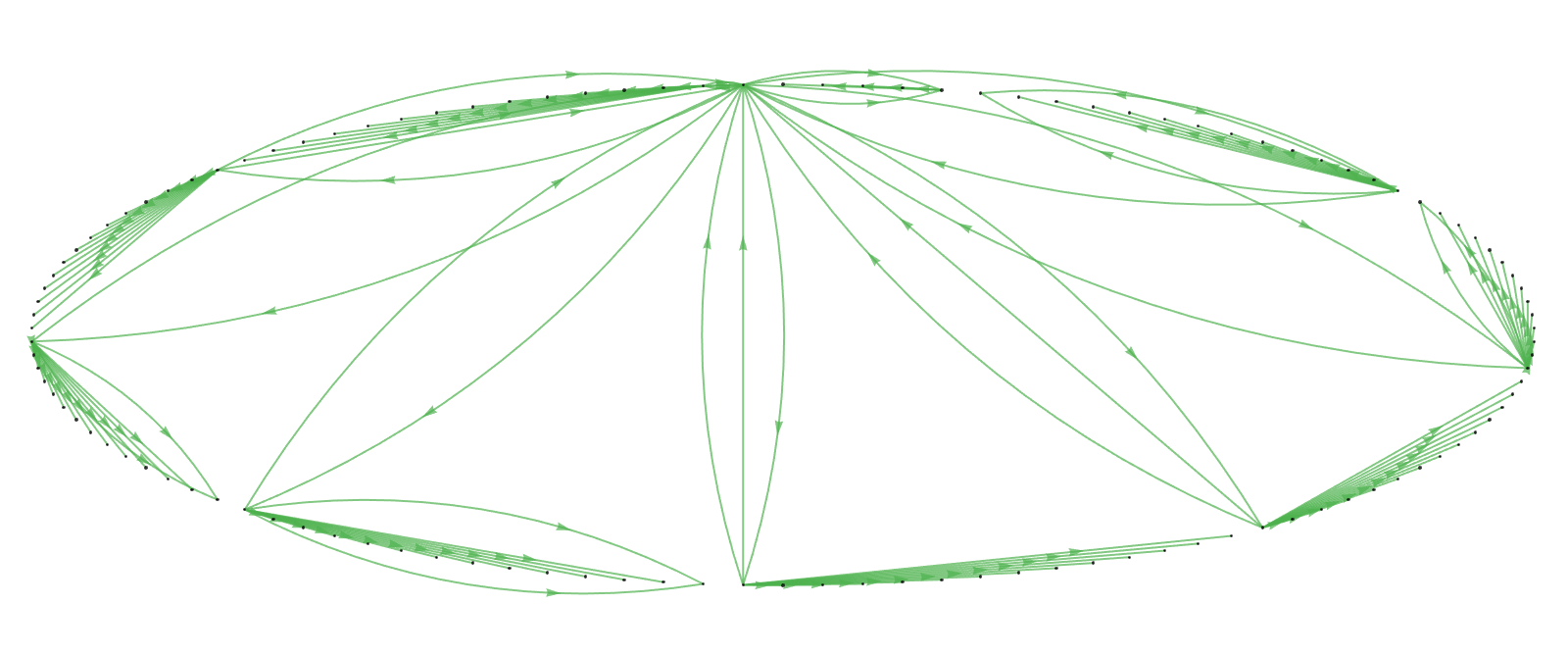
Our exploration of the Ruliad is, with a limited set of rules and computational resources, made possible by the RuliadTrotter function.
PacletInstall["https://wolfr.am/Multicomputation.paclet",
  ForceVersionInstall -> True];
<< Wolfram`Multicomputation`
axioms = {a_\[SmallCircle] (c_\[SmallCircle] b_) ->
    a\[SmallCircle] (b\[SmallCircle] c), (b_\[SmallCircle]
       a_)\[SmallCircle] c_ -> (a\[SmallCircle]b)\[SmallCircle] c,
   1\[SmallCircle]a_ -> a, a_\[SmallCircle]1 -> a,
   a_ -> a\[SmallCircle]1};
inits = {1\[SmallCircle](((1\[SmallCircle]1)\[SmallCircle]1\
\[SmallCircle]1\[SmallCircle]0)\[SmallCircle]0)\[SmallCircle]1\
\[SmallCircle]1};
trots = 2;
hgm = HypergraphMulti[inits, axioms];
hgm[
 "Graph",
 trots,
 EdgeStyle -> Directive[Thickness[0.01], RGBColor[0.4, 0.4, 0.6, 0.4]],
 GraphLayout -> "RadialEmbedding",
 VertexStyle -> RGBColor[0.2, 0.8, 0.2],
 VertexShapeFunction -> "Star",
 EdgeShapeFunction -> GraphElementData["CurvedArc"]
 ]
I found the dynamics of the Ruliad fascinating, I found them to be very kind, loyal, trusting, and affectionate; does John Wheeler's 'Really Big Questions' ring a bell? I don't want to force the comparison but there were some similarities that struck me.
Do you think it's possible to localize proper time in physics, resulting in a partially ordered set of antichains? There's already a possibility that multi-way systems in our axial dynamics could correspond to Hilbert spaces or the Curry-Howard correspondence.
PacletInstall["https://wolfr.am/Multicomputation.paclet",
  ForceVersionInstall -> True];
<< Wolfram`Multicomputation`
axioms = {
   (a_\[SmallCircle]b_)\[SmallCircle](c_\[SmallCircle]d_) -> (a\
\[SmallCircle]c)\[SmallCircle](b\[SmallCircle]d),
   a_\[SmallCircle](b_\[SmallCircle]c_) -> (a\[SmallCircle]b)\
\[SmallCircle](a\[SmallCircle]c)\[SmallCircle]c,
   1\[SmallCircle]a_ -> a,
   a_ -> 1\[SmallCircle]a,
   a_\[SmallCircle]1 -> a,
   a_ -> a\[SmallCircle]1
   };
inits = {1\[SmallCircle]((0\[SmallCircle]1)\[SmallCircle]0)};
trots = 2;
hgm = HypergraphMulti[inits, axioms];
hgm[
 "Graph",
 trots,
 EdgeStyle -> Directive[RGBColor[0.4, 0.4, 0.6, 0.4]],
 GraphLayout -> "HighDimensionalEmbedding",
 AspectRatio -> 5/9,
 VertexStyle -> Directive[RGBColor[0.6, 0.2, 0.2]]
 ]
This post really discovers the possible foliations on the corresponding causal graphs, it's a significant contribution that sheds light on the computational aspect, it's incredibly useful like the big streams of paper that go into delivering the newspapers.
Your axiom management @Aritra Sarkar is something we've never done before, there are so many tentacles.
PacletInstall["https://wolfr.am/Multicomputation.paclet",
ForceVersionInstall -> True];
<< Wolfram`Multicomputation`
axiomsSGT1 = {a_\[SmallCircle](b_\[SmallCircle]c_) -> \
(a\[SmallCircle]b)\[SmallCircle]c, \
(a_\[SmallCircle]b_)\[SmallCircle]c_ ->
a\[SmallCircle](b\[SmallCircle]c)};
inits = {1\[SmallCircle]((0\[SmallCircle]1)\[SmallCircle]0)};
trots = 2;
hgm = HypergraphMulti[inits, axiomsSGT1];
hgm["Graph", trots,
VertexShapeFunction ->
Function[{pos, v, size},
Inset[Framed[
Style[Wolfram`Multicomputation`FromLinkedHypergraph[v,
"Expression"], Bold, Gray],
FrameStyle -> {Thin, RGBColor[0.1, 0.1, 0.3],
FontColor -> RGBColor[0.58, 0.12, 0.16]}], pos, size]],
PerformanceGoal -> "Quality",
EdgeStyle -> Directive[RGBColor[0.97, 0.91, 0.54]],
GraphLayout -> "RadialEmbedding", AspectRatio -> 1/2]
hgm["CausalGraph", trots, "Expression", AspectRatio -> 3/9]
hgm = HypergraphMulti[inits, axiomsSGT1];
hgm["Graph", trots,
EdgeStyle -> Directive[RGBColor[0.38, 0.51, 0.78]],
GraphLayout -> "CircularEmbedding", AspectRatio -> 1/3]
hgm["CausalGraph", trots, VertexLabels -> None, AspectRatio -> 1/2]
axioms = {a_\[SmallCircle](b_\[SmallCircle]c_) -> (a\[SmallCircle]b)\
\[SmallCircle]c, (a_\[SmallCircle]b_)\[SmallCircle]c_ ->
a\[SmallCircle](b\[SmallCircle]c)};
inits = {1\[SmallCircle]((0\[SmallCircle]1)\[SmallCircle]0)};
trots = 2;
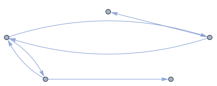
g = ResourceFunction["MultiwayOperatorSystem"][axioms, inits, trots,
"EvolutionCausalGraph", AspectRatio -> 1/3];
Show[GraphPlot[g, GraphLayout -> "Star"]]
This EvolutionCausalGraph shows how the observer perspective adapts quickly to the changing landscape of the Ruliad.
Your RuliadTrotter of the observer perspective, is not a question of specific computational knowledge; the big picture is just a question of strategic thinking whether it's the unital magma theory, the semigroup theory, the monoid theory, or even the group theory axioms.