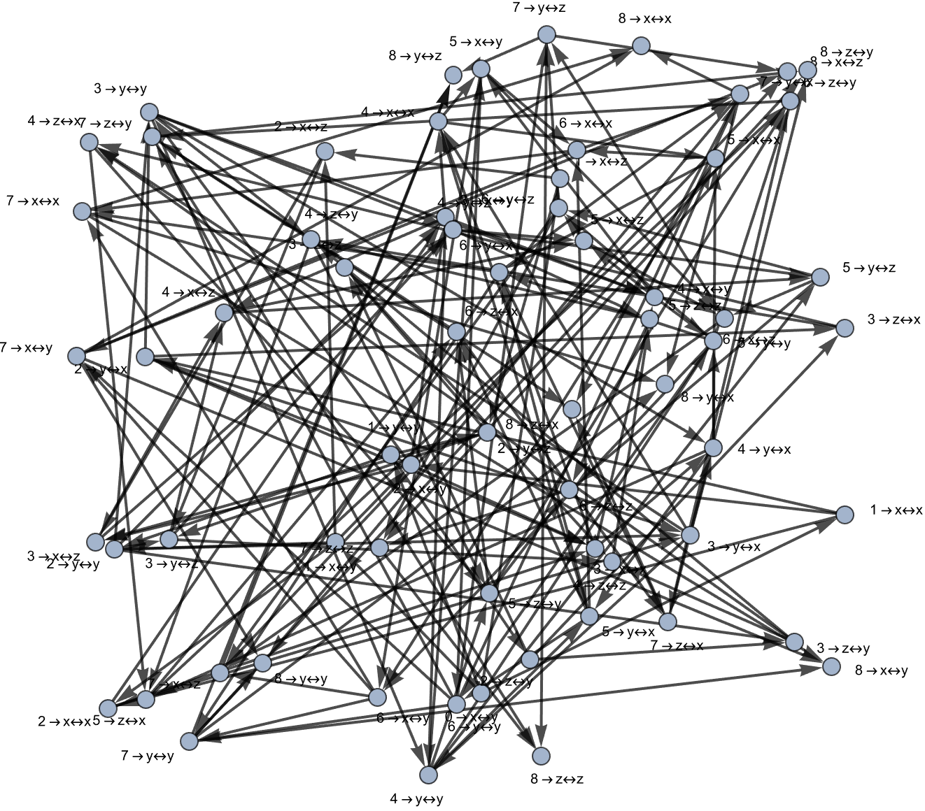
An interesting and worthwhile thing to be exposed to is a window into a different way of thinking about things; a meta-level how to think about things. Decreasingly, education teaches us to think about technical and mechanical knowledge; even fields that teach you to think about things are ground down to production, industrial line technical knowledge. What problems are worth solving ? What we should do, is we should set up the iconic, multiway system to explore all possible evolutions of the system based on rules that we have decided to define, at the moment. Each state in the system, represents a different configuration, and transitions between these states represent transformations or changes.

multiwaySystem = ResourceFunction["MultiwaySystem"];
rulesSimpleCycles = {"P" -> "Q", "Q" -> "R", "R" -> "P"};
rulesSelfLoopCycle = {"P" -> "P", "P" -> "Q", "Q" -> "R", 
   "R" -> "P"};
rulesBranchingRejoining = {"P" -> "Q", "Q" -> "R", "R" -> "P", 
   "Q" -> "S", "S" -> "P"};
rulesComplexInteractions = {"P" -> "Q", "Q" -> "R", "R" -> "P", 
   "P" -> "S", "S" -> "Q", "R" -> "T", "T" -> "P"};
generateVisualizations[rules_, steps_, title_] := 
  Module[{multiwaySystemVisual, evolutionGraphVisual, plotLabel}, 
   multiwaySystemVisual = 
    multiwaySystem[rules, "P\[LeftRightArrow]Q", steps, "StatesGraph",
      "IncludeStepNumber" -> True, GraphLayout -> "SpringEmbedding"];
   evolutionGraphVisual = 
    multiwaySystem[rules, "P\[LeftRightArrow]Q", steps + 2, 
     "EvolutionCausalGraph", "IncludeStepNumber" -> True, 
     GraphLayout -> "SpringEmbedding"];
   plotLabel = TextCell[title, "Title"];
   Column[{plotLabel, 
     Show[{multiwaySystemVisual, evolutionGraphVisual}, 
      ImageSize -> Large, 
      PlotLabel -> 
       "Causal Graph Construct Multiway Space and Evolution", 
      Frame -> True]}]];
multiwaySystemExplanation = 
  Style[TextCell[
    "By requiring proof paths to explore all possible evolutions of a \
system according to given rules, we obtain a multiway system--a \
computational model the price at which we collectively represent each \
node which represents a state, each edge which represents a \
transformation between states. This approach is really useful in \
understanding metamathematical space, where each state could be \
viewed as a theorem and each transformation, as a proof step.", 
    "Text"], RGBColor[0.1, 0.1, 0.1]];
rulesExplanationSimpleCycles = 
  Style[TextCell["Simple Cycles--the Ruler of all Multiway Systems:
  1. P -> Q
  2. Q -> R
  3. R -> P
These three rules form a simple cycle, demonstrating basic cyclic \
proof paths within the space, of metamathematics.", "Text"], 
   RGBColor[0.1, 0.1, 0.1]];
rulesExplanationSelfLoopCycle = 
  Style[TextCell["Self-Loop and then Cycle, Multiway Rules:
  1. P -> P
  2. P -> Q
  3. Q -> R
  4. R -> P
I suppose another key area that is just learning at some level is the \
cycle and self-loop, illustrating the concept of theorems that can be \
revisited, within the process of proving.", "Text"], 
   RGBColor[0.1, 0.1, 0.1]];
rulesExplanationBranchingRejoining = 
  Style[TextCell["Rejoining and Branching, in this multiway system:
  1. P -> Q
  2. Q -> R
  3. R -> P
  4. Q -> S
  5. S -> P
These rules introduce branching paths that eventually rejoin, showing \
at will how different proof paths can converge back to common \
theorems.", "Text"], RGBColor[0.1, 0.1, 0.1]];
rulesExplanationComplexInteractions = 
  Style[TextCell["A More Complex Interactive Multiway System:
  1. P -> Q
  2. Q -> R
  3. R -> P
  4. P -> S
  5. S -> Q
  6. R -> T
  7. T -> P
This is the scenario that demonstrates more complex interactions, \
wherein multiple cycles and branches interact and provide a richer \
structure of proof paths, in the space of metamathematics.", "Text"], 
   RGBColor[0.1, 0.1, 0.1]];
evolutionGraphExplanation = 
  Style[TextCell[
    "The causal relationships between states, is shown in the \
evolution causal graph above; each node represents at a particular \
step the state, and each edge shows how one state leads to another. \
This graph helps visualize the dynamic process of time-elapsed \
theorem proving, capturing the relative interactions and dynamics of \
multiple proving paths. In the following proof paths we will provide \
logical operations and their corresponding rules.", "Text"], 
   RGBColor[0.1, 0.1, 0.1]];
Column[{TextCell["Visualizing the Multiway System", "Title"], 
  multiwaySystemExplanation, rulesExplanationSimpleCycles, 
  generateVisualizations[rulesSimpleCycles, 8, "Simple Cycle"], 
  rulesExplanationSelfLoopCycle, 
  generateVisualizations[rulesSelfLoopCycle, 8, 
   "Cycle and Self-Loop"], rulesExplanationBranchingRejoining, 
  generateVisualizations[rulesBranchingRejoining, 8, 
   "Rejoining and Branching"], rulesExplanationComplexInteractions, 
  generateVisualizations[rulesComplexInteractions, 8, 
   "Complex Multiway Interactions"], 
  TextCell["Evolution Causal Graph", "Title"], 
  evolutionGraphExplanation}]

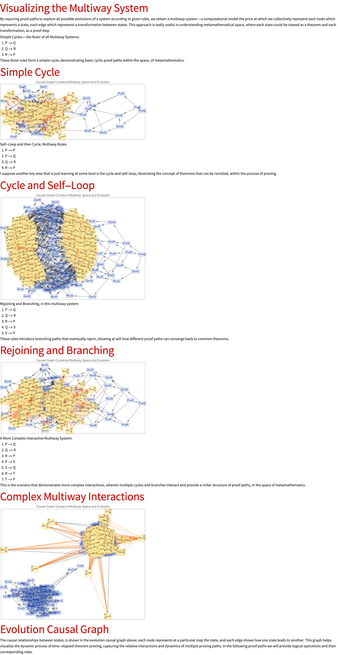
Are we visualizing the same transformation? I think the answer is considered to be yes. We always use evolution causal graphs to map the causal relationships between states over time, providing detail; there are ways to examine simple cycles, self-loops, branching paths, and even more complex interactions to illustrate the interrelated transitions and different states. What we get is a personalized pathway through which states influence one another. If the graph's big enough then that increases the probability that we can mix what we considered to be energetic, entrepreneurial kinds of graphs with scholarly graphs and in fact, each logical operation has specific rules that govern how logical statements can be transformed or simplified. Conjunction elimination is also known as simplification; that means that it accentuates the extraction from a conjunction, of either component whether it's A or B; if both A and B are true, then individually A is true, and B is true.

processLabel[label_String] := 
 Module[{coreRule}, 
  coreRule = StringReplace[label, "{" ~~ rule__ ~~ "}" :> rule];
  coreRule = StringSplit[coreRule, ","][[1]];
  coreRule]
multiwaySystem = ResourceFunction["MultiwaySystem"];
logicRules = {"A && B" -> "A", "A && B" -> "B", "A || B" -> "A", 
   "A || B" -> "B", "!A || B" -> "A -> B", "!A" -> "False", 
   "A && !A" -> "False", "False" -> "A"};
AutomatedTheoremProver[rules_List, initialState_, steps_Integer] := 
  Module[{evolutionGraph}, 
   If[! MatchQ[initialState, _String], 
    Return["Error: Initial state must be a string."]];
   If[steps <= 0, 
    Return["Error: Number of steps must be a positive integer."]];
   evolutionGraph = 
    multiwaySystem[rules, initialState, steps, "EvolutionCausalGraph"];
   evolutionGraph];
initialState = "A && B";
steps = 10;
proofGraph = AutomatedTheoremProver[logicRules, initialState, steps];
modusPonensRules = {"A && (A -> B)" -> "B"};
initialStateModusPonens = "A && (A -> B)";
steps = 10;
proofGraphModusPonens = 
  AutomatedTheoremProver[modusPonensRules, initialStateModusPonens, 
   steps];
deMorgansRules = {"!(A && B)" -> "!A || !B", 
   "!(A || B)" -> "!A && !B"};
initialStateDeMorgans = "!(A && B)";
steps = 10;
proofGraphDeMorgans = 
  AutomatedTheoremProver[deMorgansRules, initialStateDeMorgans, steps];
doubleNegationRules = {"!!A" -> "A"};
initialStateDoubleNegation = "!!A";
steps = 10;
proofGraphDoubleNegation = 
  AutomatedTheoremProver[doubleNegationRules, 
   initialStateDoubleNegation, steps];
createGraphWithProcessedLabels[proofGraph_] := 
  Module[{graph = proofGraph}, 
   If[! StringQ[graph], 
    graph = Graph[graph, 
      VertexLabels -> 
       Table[v -> processLabel[ToString[v]], {v, VertexList[graph]}], 
      VertexStyle -> LightBlue, EdgeStyle -> Gray, 
      GraphLayout -> "SpringEmbedding"]];
   graph];
Column[{TextCell["Logical Operations", "Title"], 
  Dynamic[createGraphWithProcessedLabels[proofGraph]], 
  TextCell["Modus Ponens", "Title"], 
  Dynamic[createGraphWithProcessedLabels[proofGraphModusPonens]], 
  TextCell["De Morgan's Law", "Title"], 
  Dynamic[createGraphWithProcessedLabels[proofGraphDeMorgans]], 
  TextCell["Double Negation Elimination", "Title"], 
  Dynamic[createGraphWithProcessedLabels[proofGraphDoubleNegation]]}]

Conjunction Elimination describes the operation of Logical AND that is A && B. The thing that I realized is that A && B -> A and A && B -> B. And then I realized actually! That we can have Disjunction Elimination which simplifies a disjunction by considering each disjunct separately. We can simply discard A or B given the other is true. It's a colorful way to focus on each possible case in a more simplistic manner. We also have implication, which can be expressed as !A || B. This rule redefines the implication in terms of negation and disjunction, for which the classical logic definitions decisively align. What about Negation and Contradiction? Well, negation of a proposition !A is like saying that False indicates that A must be true to avoid contradiction. How can it be that !A leads to a contradiction? How does the conjunction of a proposition and its negation A && !A result in False? That's the Rule of Contradiction. Ex Falso Quodlibet - from a contradiction False, any proposition A can follow, demonstrating that contradictions lead out to logical inconsistency.

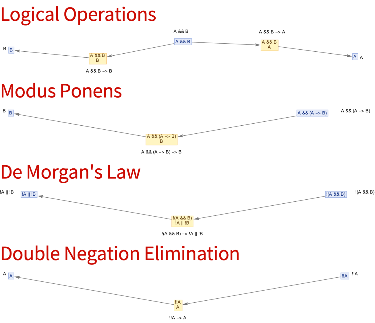
Modus Ponens is an operation that first and foremost infers B from A and then maybe A -> B. It's a nice way of teaching that A && (A -> B) -> B. It allows one to infer that B if A is true and A implies B. In professional, propositional logic we have something called De Morgan's Law, which is like saying that !(A && B) -> !A || !B while !(A || B) -> !A && !B. And if that means what we've got on the graphs which is that we can distribute negation over conjunctions and disjunctions, then yes we can simplify negation to said expressions. We also introduce Double Negation Elimination, with which the operation of !!A is doing what we think is !!A -> A and which states that negating a negation returns the original proposition; that is how double negation elimination formalizes the idea that !!A simplifies to A.

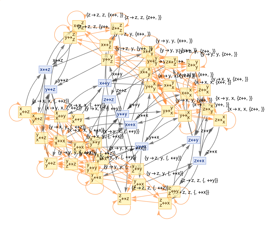
Now at least at the present time we have generated proof graphs, the morning flower that serves as the fountainhead of our conceptualization of what it means to switch gears to our multiway system. And so we started out with this non-trivial fact..the equivalence between inertial and gravitational mass is a big feature of general relativity, the principle of equivalence that was developed in 1915, by Einstein and actually, in our models (the physics) it is inevitably true..in the framework for thinking about spacetime that general relativity has. In metamathematical space, we've got this theoretical construct that is designed to "replace" the universe of mathematical theorems and proofs. And that's the only way that I can get the thing to not accelerate, if one hand was pushing harder than the other with more force I would start accelerating in a particular direction. With every action there's an equal and opposite reaction. Look at all those Klein groups! The red figures really represent a lot of stuff like the structural and categorical aspects, of meta-mathematical space.

AutomatedTheoremProver[rule_, startState_, steps_] := 
  ResourceFunction["MultiwaySystem"][rule, startState, steps, 
   "EvolutionCausalGraph"];
rules = {"x" -> "y", "y" -> "x", "y" -> "z", "x" -> "x", "y" -> "y", 
   "z" -> "z"};
proofGraph = 
  AutomatedTheoremProver[rules, "x\[LeftRightArrow]y", 10];
Graph[proofGraph, VertexLabels -> "Name", VertexStyle -> LightBlue, 
 EdgeStyle -> Gray, GraphLayout -> "SpringEmbedding"]
CategoryExample := 
 Graph[{a -> b, b -> c, c -> a}, VertexLabels -> "Name", 
  VertexStyle -> LightGreen, EdgeStyle -> Black, 
  GraphLayout -> "CircularEmbedding"]
CategoryExample
ParallelMap[AutomatedTheoremProver[rules, #, 6] &, {"x", "y", "z"}]
CategorifyTheoremProving[axioms_] := 
  Module[{categoryRules}, 
   categoryRules = Map[# -> (#[[1]] <> #[[2]]) &, Tuples[axioms, 2]];
   DirectedGraph[Graph[categoryRules, VertexLabels -> "Name"]]];
axiomsExample = {"A", "B", "C"};
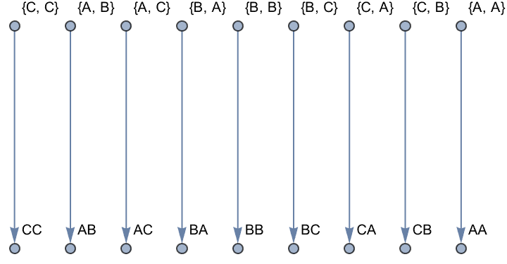
CategorifyTheoremProving[axiomsExample]
CausalityGraph[rule_, startState_, steps_] := 
  ResourceFunction["MultiwaySystem"][rule, startState, steps, 
   "CausalGraph"];
causalityExample = CausalityGraph[rules, "x\[LeftRightArrow]y", 8];
Graph[causalityExample, VertexLabels -> "Name", 
 VertexStyle -> LightRed, EdgeStyle -> Gray, 
 GraphLayout -> "SpringEmbedding"]

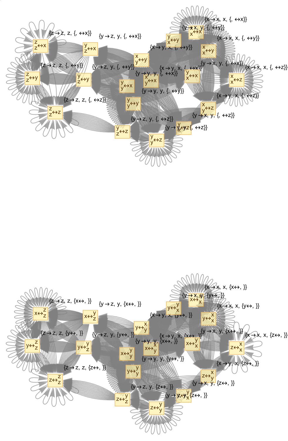
In other words, you just have to talk about the motion of that object you don't have to talk about what that object is doing. Traditionally, Automated Theorem Proving refers to systems that prove pre-defined theorems. And describe how everything fits together, automated theorem generators that aim to discover all possible theorems from a set of axioms. The law of friction says there's a force..visual representations of theorems as vertices and their logical connections (proofs) as edges. So when you do that three-point sequence within the entailment structure, when you put that into Newton's laws of motion what it's going to say is that there's a progression from axioms to the conclusion of a theorem. Usually it takes me decades to have these different ATPs working in parallel so considering the computational resources there must be a conspiracy, in reaching the conclusions..ordinary friction is about solid surfaces rubbing against each other. The introduction of a temporal dimension to account for the dynamic process of theorem proving, is exponentially essential for throwing a ball in space or on the moon.

basicRules = {"x" -> "y", "y" -> "x", "y" -> "z", "x" -> "x", 
   "y" -> "y", "z" -> "z"};
multiwayEvolution = 
  ResourceFunction["MultiwaySystem"][basicRules, 
   "x\[LeftRightArrow]y", 3, "EvolutionCausalGraph", 
   "IncludeStepNumber" -> True, GraphLayout -> "SpringEmbedding"];
newtonianProofModel = 
  ResourceFunction["MultiwaySystem"][{"x" -> "y + t", "y" -> "x - t", 
    "y" -> "z * t"}, "x\[LeftRightArrow]y", 3, "EvolutionCausalGraph",
    "IncludeStepNumber" -> True, GraphLayout -> "SpringEmbedding"];
einsteinianModel = 
  ResourceFunction["MultiwaySystem"][{"x" -> "y/c^2", "y" -> "x*c^2", 
    "y" -> "z/c"}, "x\[LeftRightArrow]y", 3, "EvolutionCausalGraph", 
   "IncludeStepNumber" -> True, GraphLayout -> "SpringEmbedding"];
causalityGraph = 
  ResourceFunction["MultiwaySystem"][basicRules, 
   "x\[LeftRightArrow]y", 3, "CausalGraph", 
   "IncludeStepNumber" -> True, GraphLayout -> "SpringEmbedding"];
GraphicsGrid[{{multiwayEvolution, 
   newtonianProofModel}, {einsteinianModel, causalityGraph}}, 
 Frame -> All]

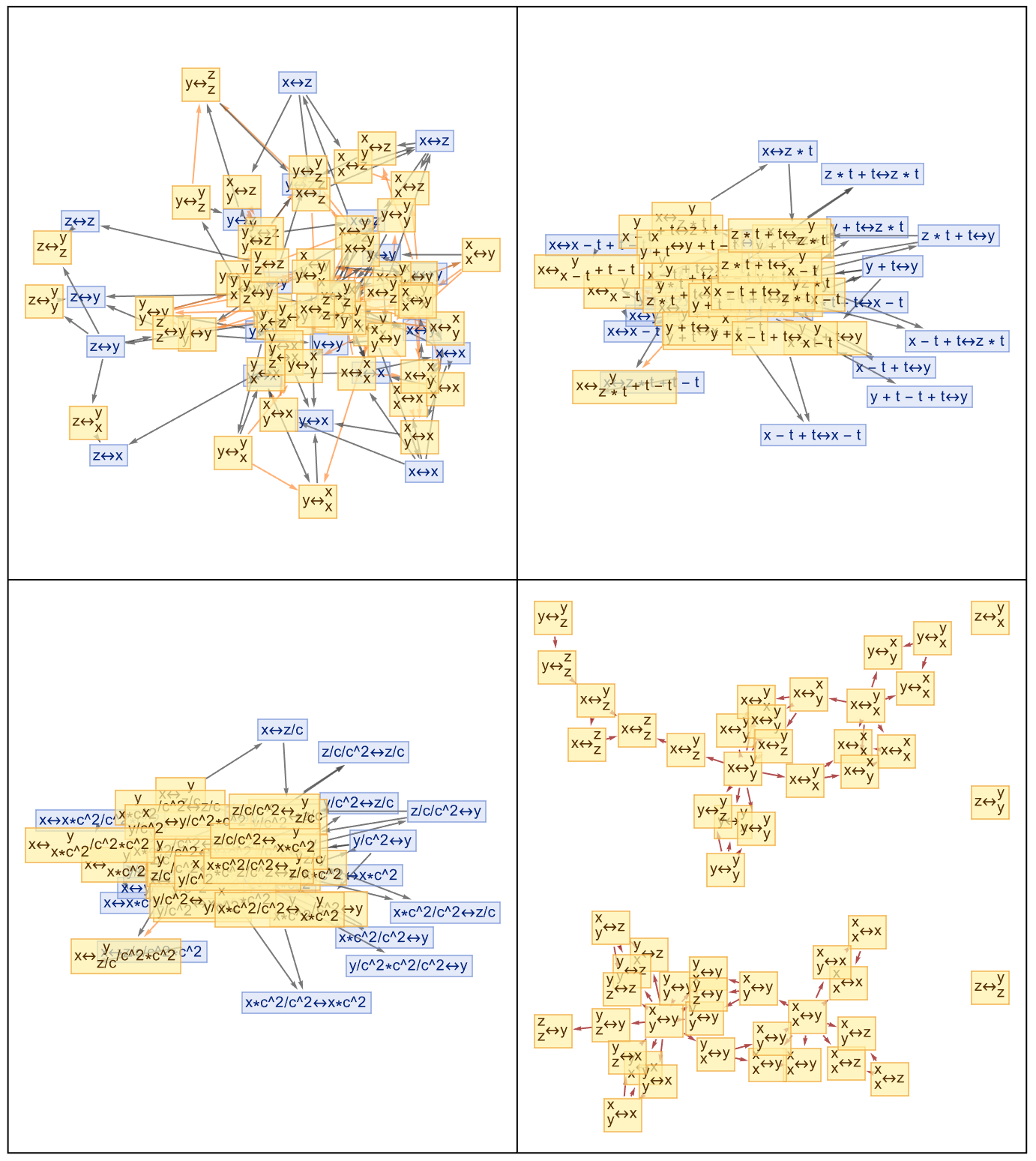
You throw a ball in the air it has a certain drag, I should explain that um, the amount of drag..there are four parameters that affect the actual force on an object going through air or water or gas or a liquid. How big is the object? What is the density of the material; like air, water has a higher density, how big is the object what is the density of the material, how fast is the object going? What is viscosity? Viscosity is a little bit like a coefficient of friction but it isn't defined the same way at all..there's an analogy to physics: the transition from spatial trajectories to spacetime worldlines. And last but not least what you're really doing is, the inclusion of all possible worldlines or paths that ATPs can take. Because then what we can do is map out everything, we can reach the centennial and so when you try and pour it you've got that jug or something, you're trying to get that liquid to fall out of the jug, when you have viscosity it flows less easily. That means the concept of "event horizons" and the limits of theorem proving within this framework...show how metamathematical concepts can shine through as we ride off into the sunset. There must be a Wolfram Language extension that adds extended keywords like the quantity, the speed of the object, the density, and the viscosity of the fluid it's going through. And those are the only things that the drag on an object can depend on.

rules = {"x" -> "y", "y" -> "x", "y" -> "z", "x" -> "x", "y" -> "y", 
   "z" -> "z"};
multiwaySystem = 
  ResourceFunction["MultiwaySystem"][rules, "x\[LeftRightArrow]y", 6, 
   "StatesGraph", "IncludeStepNumber" -> True, 
   GraphLayout -> "SpringEmbedding"];
causalGraph = 
  ResourceFunction["MultiwaySystem"][rules, "x\[LeftRightArrow]y", 6, 
   "CausalGraph", "IncludeStepNumber" -> True, 
   GraphLayout -> "SpringEmbedding"];
categoryExample = 
  Graph[VertexList[multiwaySystem], EdgeList[multiwaySystem], 
   VertexLabels -> "Name", EdgeLabels -> "Name"];
automatedTheoremProving[category_, theorem_] := 
  Module[{proofs}, 
   proofs = 
    FindPath[category, First[theorem], Last[theorem], {Infinity}, All];
   If[Length[proofs] > 0, "Theorem Proved", "Theorem Not Proved"]];
{multiwaySystem, causalGraph, categoryExample}

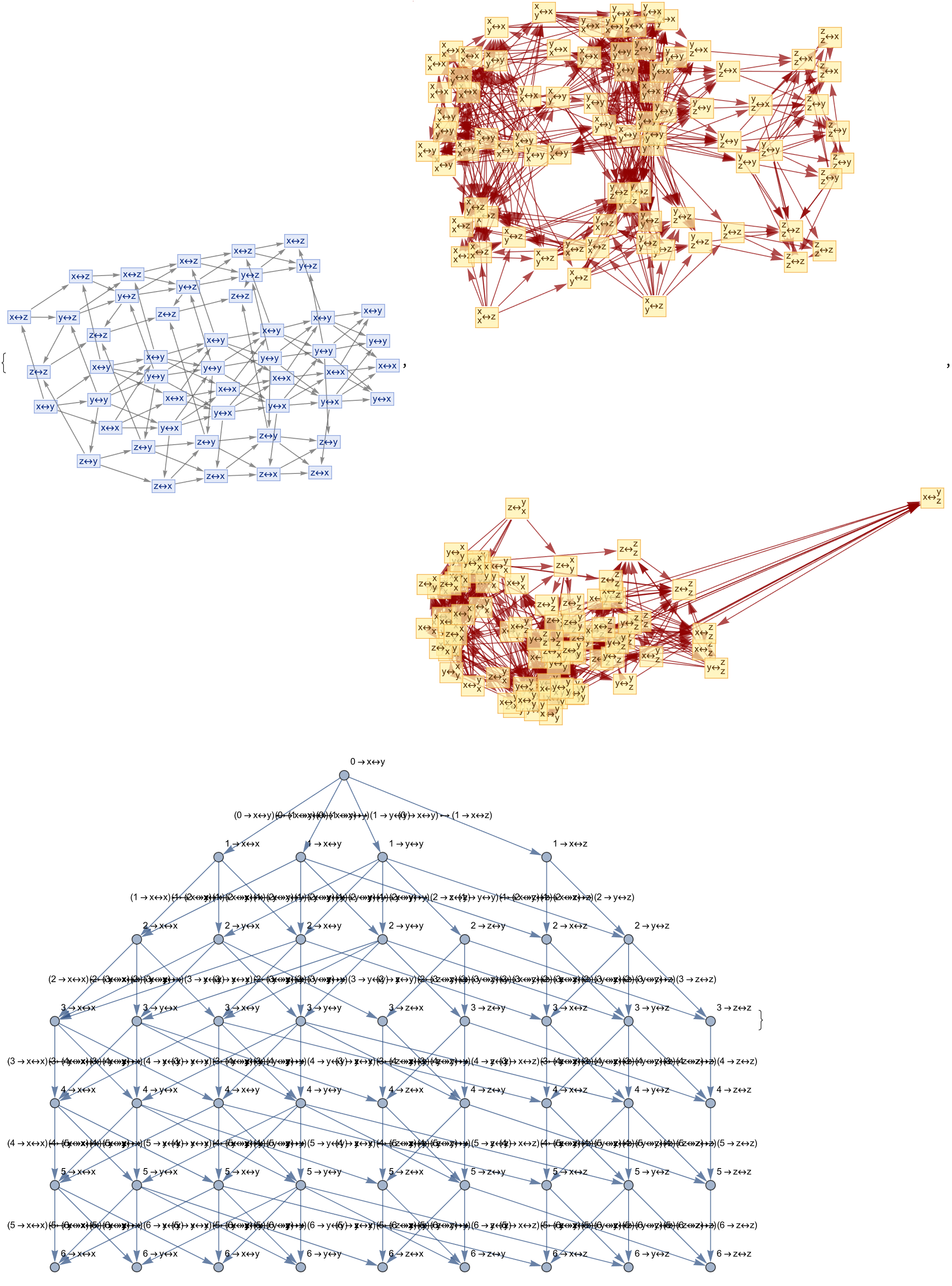
There's just one way of combining those quantities it's called the Reynold's number and let's see, what is it? Uh buh buh buhhh it's size times velocity divided by viscosity over density, if I remember correctly. And that, is how we explore metamathematical concepts with or without you, how they differ from category theory. It's the way that structures in metamathematical space can be interpreted within categorical frameworks, and that's why I'm telling you all about this stuff; so that you can look at something really big like a ship and compare the flow behind a ship a flow behind an airplane - the structure of theorem spaces may reveal deeper semantic relationships. That's why I'm here to show you all this stuff about how we extract categorical properties (objects, morphisms) from the theorems and proofs in metamathematical space.

rules = {"x" -> "y", "y" -> "x", "y" -> "z", "x" -> "x", "y" -> "y", 
   "z" -> "z"};
multiwaySystem = 
  ResourceFunction["MultiwaySystem"][rules, "x\[LeftRightArrow]y", 6, 
   "StatesGraph", "IncludeStepNumber" -> True, 
   GraphLayout -> "SpringEmbedding"];
causalGraph = 
  ResourceFunction["MultiwaySystem"][rules, "x\[LeftRightArrow]y", 6, 
   "CausalGraph", "IncludeStepNumber" -> True, 
   GraphLayout -> "SpringEmbedding"];
categoryExample = 
  Graph[VertexList[multiwaySystem], EdgeList[multiwaySystem], 
   VertexLabels -> "Name", EdgeLabels -> "Name"];
automatedTheoremProving[category_, theorem_] := 
  Module[{proofs}, 
   proofs = 
    FindPath[category, First[theorem], Last[theorem], {Infinity}, All];
   If[Length[proofs] > 0, "Theorem Proved", "Theorem Not Proved"]];
{multiwaySystem, causalGraph, categoryExample}

Stokes's law says that, let's see if I can get it right..the utilization of Wolfram tools like TwoWayRuleNestGraph and MultiwaySystem allows us to visualize and explore these concepts..and the creation of complex graphs that you've got, and the drag force is proportional to the speed at which the thing is going through the fluid...the specific examples (like the Klein group and its representations) might illustrate if you cross your eyes at it it reminds you of dropping something out of an airplane, it'll fall through the air, you do skydiving you fall through the air at a certain speed and there's a drag force. Visual representations, aid in understanding the intricate relationships and structures that we should bridge gaps, between automated theorem proving, and how fast you're falling if there wasn't any air there.

newRules = {"a" -> "b", "b" -> "a", "c" -> "a", "d" -> "c", 
   "e" -> "d", "f" -> "e"};
multiwaySys = 
  ResourceFunction["MultiwaySystem"][newRules, "a\[LeftRightArrow]b", 
   10, "EvolutionCausalGraph", "IncludeStepNumber" -> True, 
   GraphLayout -> "SpringEmbedding"];
toyCategory = 
  Graph[{1 -> 2, 2 -> 3, 3 -> 1, 1 -> 1, 2 -> 2, 3 -> 3}, 
   VertexLabels -> "Name", GraphLayout -> "CircularEmbedding"];
parallelATP = 
  Function[{rules, initial, steps}, 
   ParallelTable[
    ResourceFunction["MultiwaySystem"][rules, initial, i, 
     "StatesGraph"], {i, steps}]];
parallelProofs = parallelATP[newRules, "a\[LeftRightArrow]b", 5];
categorifyProofPaths = 
  Function[graph, Module[{edges, vertices}, edges = EdgeList[graph];
    vertices = VertexList[graph];
    Graph[edges, 
     VertexLabels -> 
      Table[v -> "Category" <> ToString[v], {v, vertices}], 
     GraphLayout -> "LayeredDigraphEmbedding"]]];
{multiwaySys, toyCategory, parallelProofs}

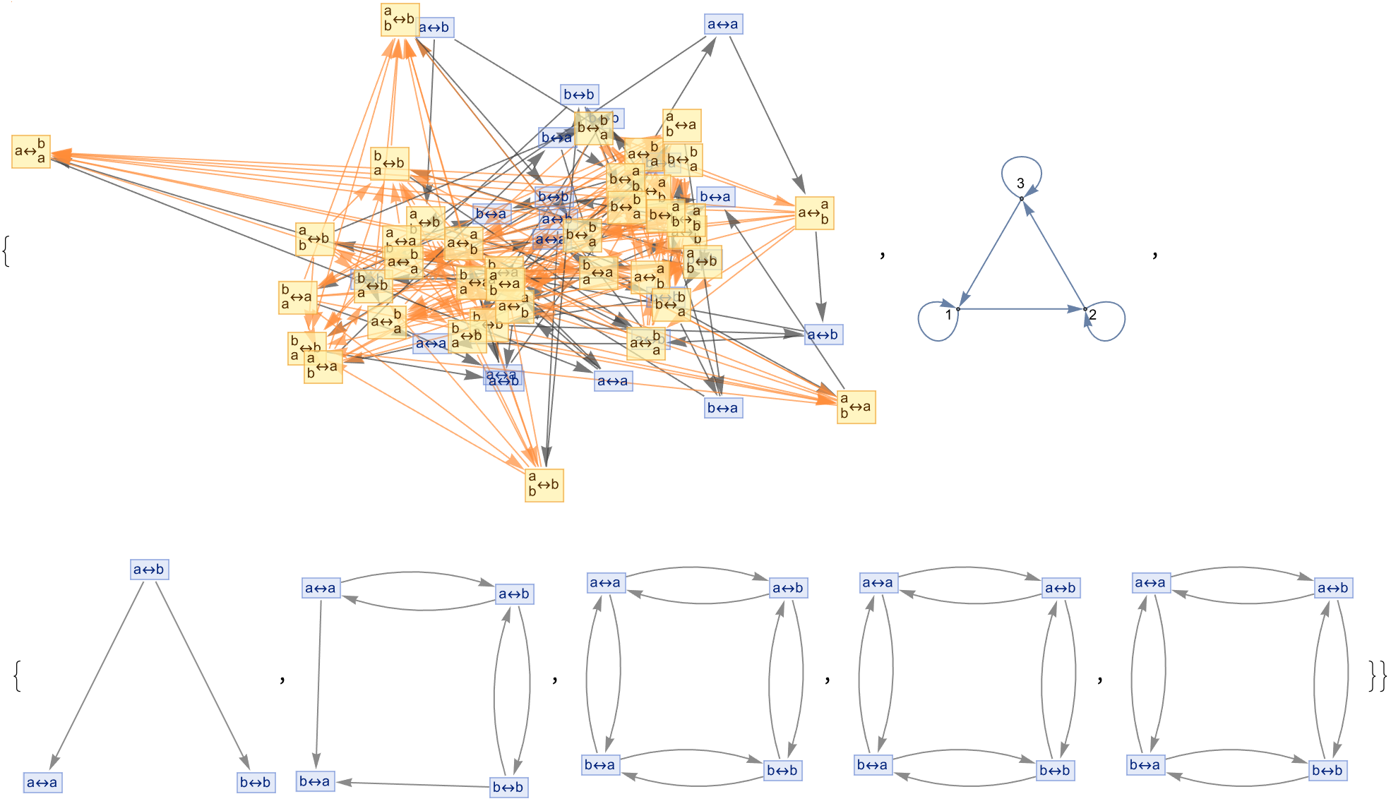
Maybe all these metamathematical proofs and category theory, they show the real purpose of algebra - it's to use Wolfram tools and technology; it provides a unique lens through which these abstract concepts can be visualized and better understood, whether it's possible to be nondeterministic or partially observable; it means this and that is a contingency problem wherein new information is provided by percepts. The solution is a plan that is based on contingencies..it should, or should it, be called the contingency plan or the plan of contingencies, we don't know what that means. There's also the unknown state space. It's not so much about the applications of avenues for further research as it is about the semantics of mathematical structures! And the potential computational applications in theorem proving and mathematical exploration. Everything that is contained within the rich and complex ideas presented by Łukasz Majsiak, each practical component of the discussion and its Wolfram implementations in metamathematical space..you'll see how it shows the fundamental structures and processes underpinning mathematics and computation.

SimpleGraph[ResourceFunction[
ResourceObject[<|
      "Name" -> "TwoWayRuleNestGraph", "UUID" -> 
       "98cc7a51-abf1-4f9f-a0dd-542056ccad73", "ResourceType" -> 
       "Function", "ResourceLocations" -> {
CloudObject[
         "https://www.wolframcloud.com/obj/wolframphysics/Resources/\
98c/98cc7a51-abf1-4f9f-a0dd-542056ccad73"]}, "Version" -> None, 
       "DocumentationLink" -> 
       URL[
        "https://www.wolframcloud.com/obj/wolframphysics/\
TwoWayRuleNestGraph"], "ExampleNotebookData" -> Automatic, 
       "FunctionLocation" -> 
       CloudObject[
        "https://www.wolframcloud.com/obj/wolframphysics/Resources/\
98c/98cc7a51-abf1-4f9f-a0dd-542056ccad73/download/DefinitionData"], 
       "ShortName" -> "TwoWayRuleNestGraph", "SymbolName" -> 
       "FunctionRepository`$98cc7a51abf14f9fa0dd542056ccad73`\
TwoWayRuleNestGraph"|>]][
    x_\[SmallCircle]y_ <-> (y_\[SmallCircle]x_)\[SmallCircle]y_, #, 2,
     AspectRatio -> 1/4, VertexStyle -> _ -> FontSize -> 13], 
   GraphLayout -> "SpringElectricalEmbedding", 
   VertexShapeFunction -> "ConcaveDiamond"] & /@ 
 Flatten[
   Groupings[#, SmallCircle -> 2] & /@ 
    Table[Tuples[{a, b, c}, n], {n, 3}]][[4 ;; 66]]

When it bounces back how much does it bounce when it bounces? That's not something you can deduce from Newton's laws alone..even then you can't compute it you pretty much just have to measure it nowadays; A New Kind of Science with physics, the problem with explaining physics is that there are things that are very clear-cut and well-understood that you'll find on textbooks on high-school physics and there are some things that may not be understood; you can apply Newton's laws and that's great except you've got this coefficient of restitution and what is that? It's not sort of clear-cut high-school level physics. And that's what it was like when I whirled multiway graphs around; metamathematics as a meta-level concept was my centrifugal force that comes from the Latin: to run away from. Running away from the center force so the, thing is effectively pulling away from you. You could asymptotically generate the space of all true theorems, from the axioms, with edges being re-writings of theorems according to the fixed set of axioms. I had so much fun with the red figures, and the rendering! because you're finding the axiomatic side of our universal computation.

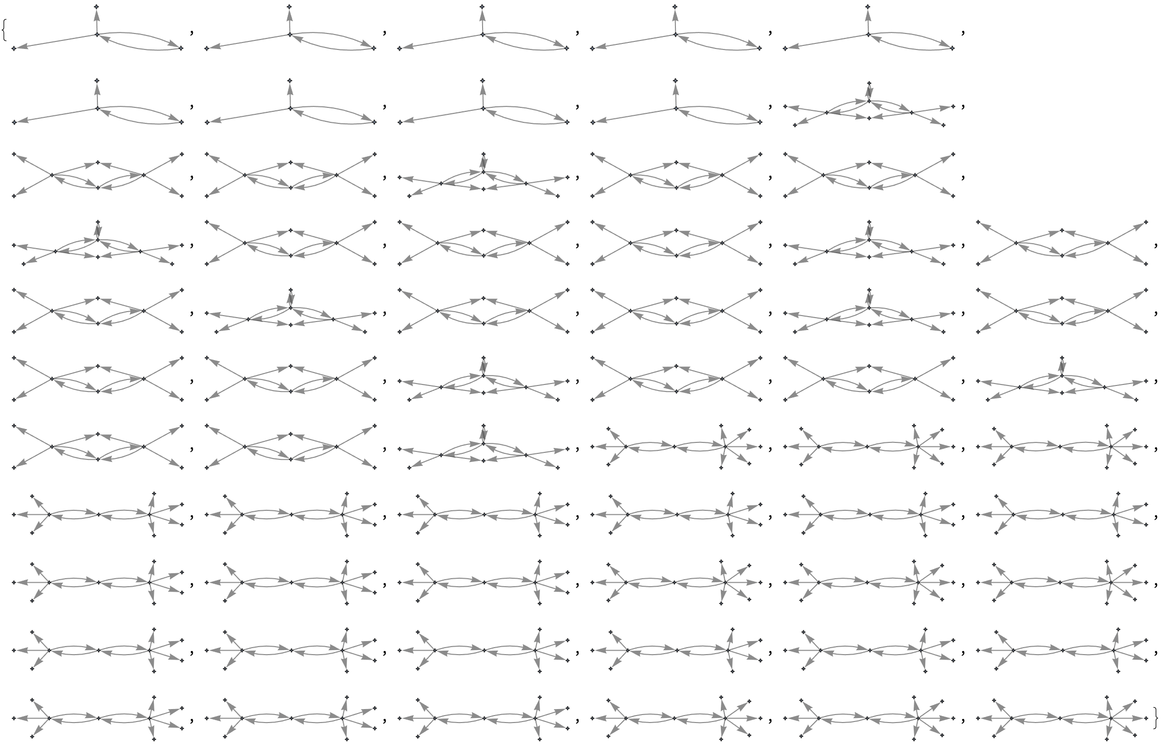
And uh, this all gets very confusing. First point. And the second point. I'm not always right; the multiway graphs that were already there, serve as tools to visualize metamathematical structures. It's like when I constructed these graphs and opened the door and it was you I didn't recognize rolling around in mathematical statements and the operations like substitution. Our mathematical operations..were pretty vigorous; when I saw that the commutativity, the illustration by the axiom a of b = b of a, and came to the conclusion that the multiway graph generated from this axiom using substitution represents Boolean hypercubes, it really demonstrated how you feel: automated theorem proving means what is usually meant by it in the literature; in your literature, it's what generates the pictures of entailment cones & categories.

ResourceFunction["MultiwaySystem"][{"x" -> "y", 
  "y" -> "x"}, "x\[LeftRightArrow]y", 6, "StatesGraph", 
 "IncludeStepNumber" -> True, 
 GraphLayout -> "SpringElectricalEmbedding"]

And that's why if you want to keep the thing going in a circle, the circuitous associativity, and that's the demonstration that we get it's like the axiom of (a of b) of c = a of (b of c), leading to simple ring-like multiway graphs. Okay so, I've gotta go! Back to my day job, in interstellar space, nowhere near any planets or stars or anything like that it's just going to keep going in a straight line - that's Newton's first law. So far, so good. And I can just stay really basic, when both associativity and commutativity are applied, the resulting multiway graph will represent a commutative semigroup: this meaning within the meaning has got us seeing double. This is our understanding of the proof paths, that are shattered across the Klein space being four-fold.

ResourceFunction["MultiwaySystem"][{"x" -> "y", "y" -> "x", 
  "y" -> "z", "x" -> "x", "y" -> "y", 
  "z" -> "z"}, "x\[LeftRightArrow]y", 6, "StatesGraph", 
 "IncludeStepNumber" -> True, 
 GraphLayout -> "SpringElectricalEmbedding"]

The acceleration that comes from the force being exerted by gravity, the acceleration needed to just, slip around Earth in orbit..if you're going at that speed you will be..the force of gravity just matches what you need to change your velocity so you just keep going around the Earth. That's how the semigroup dynamic develops, it's a concept of circular motion in that by considering specific relations or generators, such as a of a = a and b of b = b, the resulting multiway graph reveals different equivalence classes and usually the force of gravity just, pulls things right to the center like on the Earth, on the first approximation, it's not precisely the center of the Earth usually one in a thousand..the density of the rock and so on, I saw it. That's the blind spot of our specific theorems, effectively. And there's so much more. We've only got what, four red figures? Whatever that is...

ResourceFunction["MultiwaySystem"][{"x" -> "y", "y" -> "x", 
  "y" -> "z", "z" -> "x"}, "x", 8, "StatesGraph", 
 "IncludeStepNumber" -> True, 
 GraphLayout -> "SpringElectricalEmbedding"]

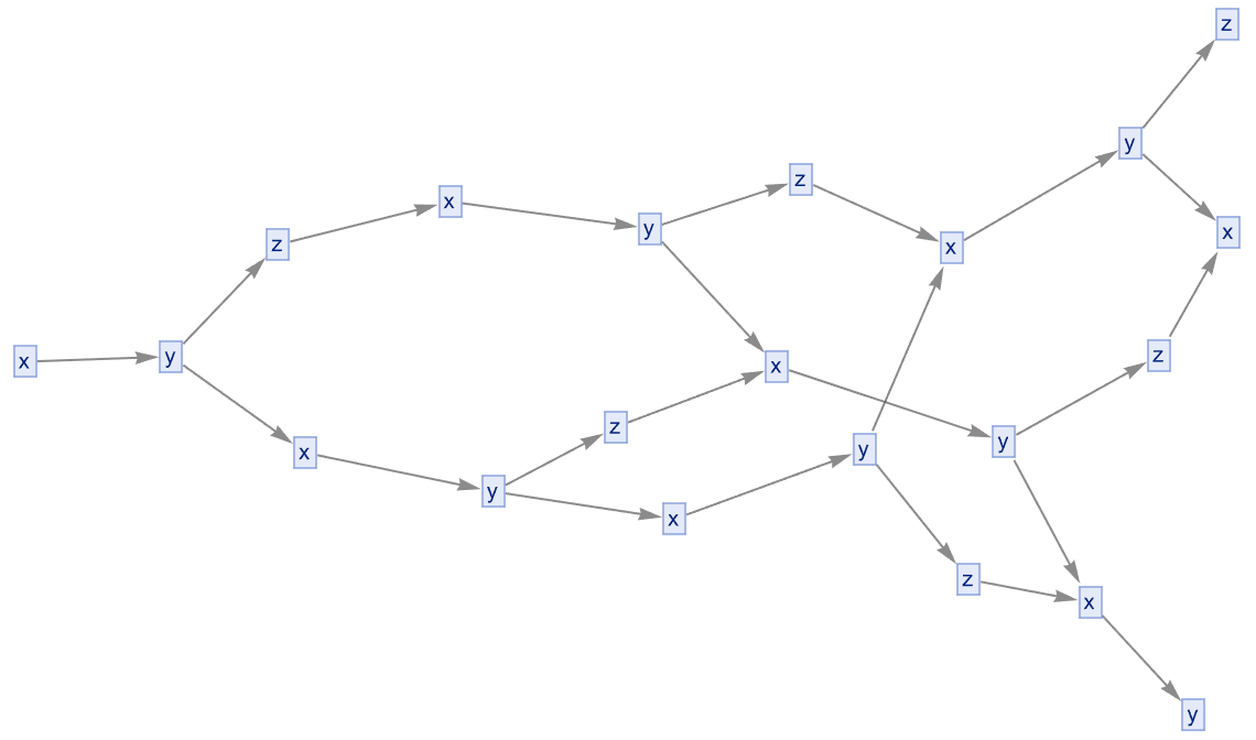
Because a black hole, it's like having a perfect sphere; you can't, it's not doing anything for us. There's a sphere there. You have to have some bit on the surface that you say oh okay that moved around. It's so great that you've got the double multi-way meaning graph that reveals different equivalence classes..these ring true for that semigroup. and It's a way to have the symbolic computation, what with all these comments that we want to make..what if we wanted the code to be the paragraph and the paragraph to be the code? How can this be? We started out with one sentence about the novel approaches, no, the whole paragraph: the construction of metamathematical space. When you see the register...for a second there I thought that the theorems were the vertices and the edges were rewritings of theorems, according to the axioms fixed in space.

rules = {"x" -> "y", "y" -> "x", "y" -> "z", "x" -> "x", "y" -> "y", 
   "z" -> "z", "x" -> "z"};
ResourceFunction[
  "MultiwaySystem"][rules, "x\[LeftRightArrow]y", 8, \
"EvolutionGraphStructure", VertexStyle -> Red, EdgeStyle -> Blue]

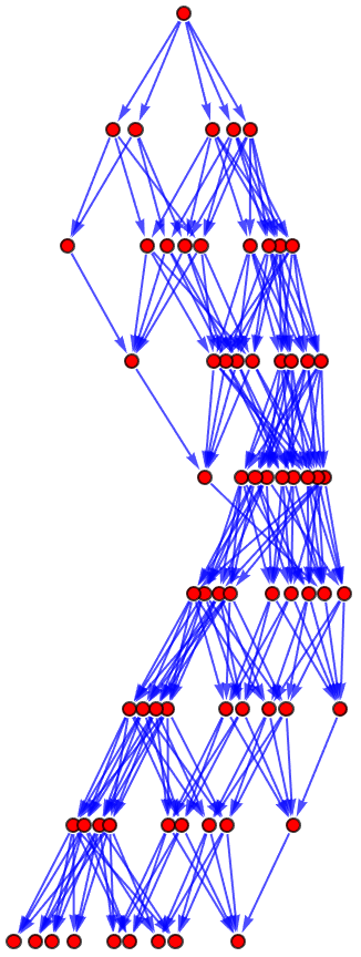
So photons or particles of light, they have, well they have zero mass but they can have a certain energy. Photons can orbit black holes. It's a massive object orbiting this massive planet..investigating products of elements in a semigroup and how they interact. If there's one thing I want, I want to see you identifying distinct elements in the semigroup by analyzing disconnected components in the multiway graphs. With small rules like this guy, don't touch this.. this is how we got into proof construction. Now we can make special, computationally irreducible time loops and serve them up on the standard entailment graph..we got every theorem in our physics project.

generateCausalGraph := 
  Function[{rules, start, steps}, 
   ResourceFunction["MultiwaySystem"][rules, start, steps, 
    "EvolutionCausalGraph", "IncludeStepNumber" -> True, 
    GraphLayout -> "SpringEmbedding"]];
causalGraph = 
  generateCausalGraph[multiwayRules, "x\[LeftRightArrow]y", 10];
Show[causalGraph, ImageSize -> Large]
automatedTheoremProving := 
  Function[{axioms, theorems}, 
   ParallelMap[FindEquationalProof[#, axioms] &, theorems]];
axiomsForProof = {x \[LeftRightArrow] y -> z \[LeftRightArrow] x};
theoremsForProof = {x \[LeftRightArrow] y == y \[LeftRightArrow] x, 
   z \[LeftRightArrow] x == x \[LeftRightArrow] z};
proofs = automatedTheoremProving[axiomsForProof, theoremsForProof];
TableForm[proofs, TableHeadings -> {None, {"Theorem", "Proof"}}]

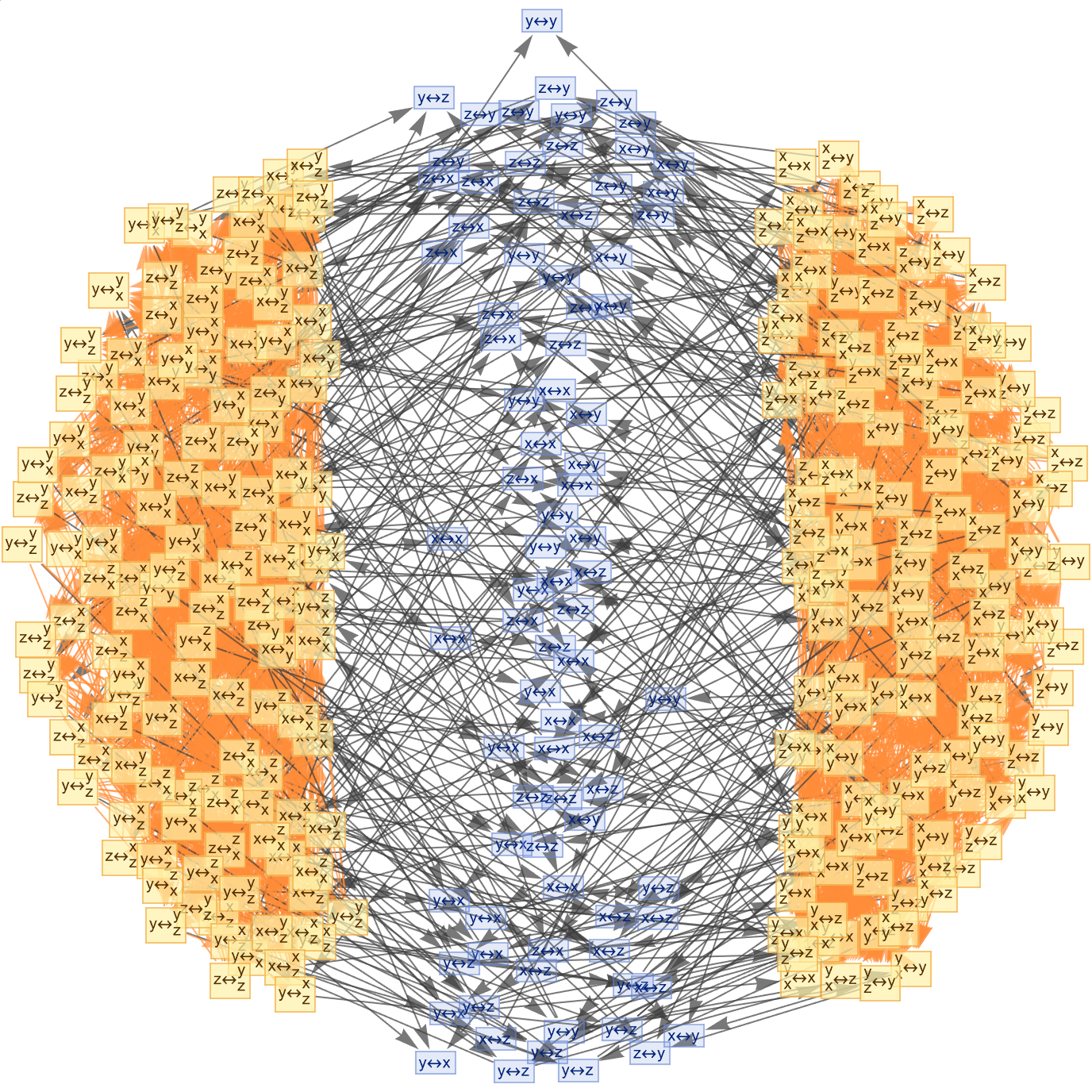
I call this the 15th image, because it's not so bad. We did it, we finally found the specific relations that lead to more equivalences and potentially infinite multiway graphs, which signifies the adjacent, infinite equivalences between expressions. And the study of these graphs allows against the identification of distinct elements or "droplets" in the semigroup, and you can work out the mechanics around that. Another area is optics, properties of light? There's a bunch you can see easily..corresponding to clusters of equivalent words with something like lenses; light is bent, the speed of light is different around the glass than it is in a vacuum. In at least certain simple certain cases..the investigation is much more complicated than elementary physics, the refractory index of water is 1.33..if we assume that light goes 1.33 times slower in water than it does in air then we can make certain conclusions about optics from that. There's a lot you can work out in optics where you're just following simple formulas and so on.

rules = {"x" -> "y", "y" -> "x", "y" -> "z", "x" -> "x", "y" -> "y", 
   "z" -> "z"};
multiwaySystem = 
  ResourceFunction["MultiwaySystem"][rules, "x\[LeftRightArrow]y", 8, 
   "StatesGraph", "IncludeStepNumber" -> True, 
   GraphLayout -> "LayeredDigraphEmbedding"];
Show[multiwaySystem]
objects = VertexList[multiwaySystem];
morphisms = EdgeList[multiwaySystem];
categoryGraph = 
  Graph[objects, morphisms, VertexLabels -> "Name", 
   EdgeLabels -> "Name", GraphLayout -> "SpringEmbedding", 
   EdgeStyle -> Directive[Blue, Arrowheads[0.03]], VertexStyle -> Red];
Show[categoryGraph]
theorem = "x" -> "z";
highlightedPaths = 
  HighlightGraph[multiwaySystem, 
   Style[PathGraph[#], Thick, Red] & /@ provingPaths];
Show[highlightedPaths]
spacetimeStructure = 
  Graph[objects, morphisms, 
   VertexCoordinates -> RandomReal[{-1, 1}, {Length[objects], 2}], 
   VertexLabels -> "Name", EdgeStyle -> Gray];
newtonianSpacetime = 
  SetProperty[
   spacetimeStructure, {GraphLayout -> "SpringEmbedding", 
    EdgeStyle -> Directive[Dashed, Gray]}];
Show[newtonianSpacetime]
einsteinianSpacetime = 
  SetProperty[
   spacetimeStructure, {GraphLayout -> "SpringEmbedding", 
    EdgeStyle -> Directive[Thick, Black]}];
Show[einsteinianSpacetime]
theorems = {"x" -> "y", "y" -> "z", "z" -> "x"};

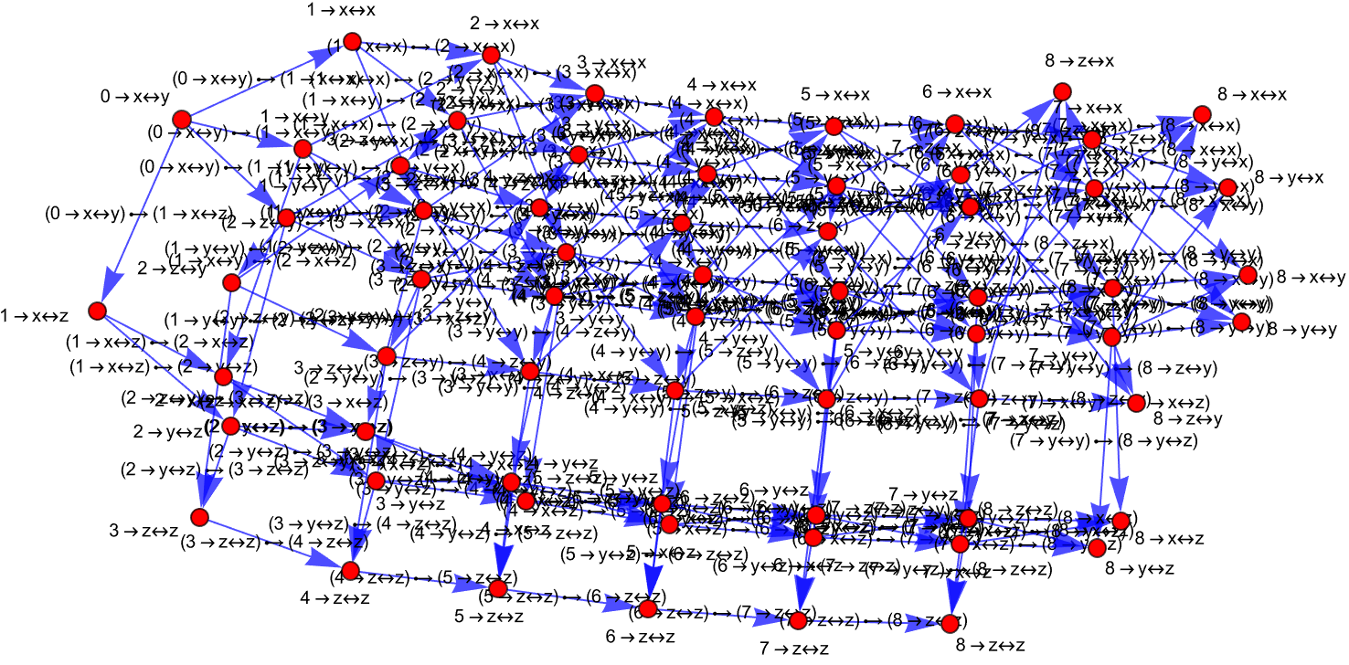
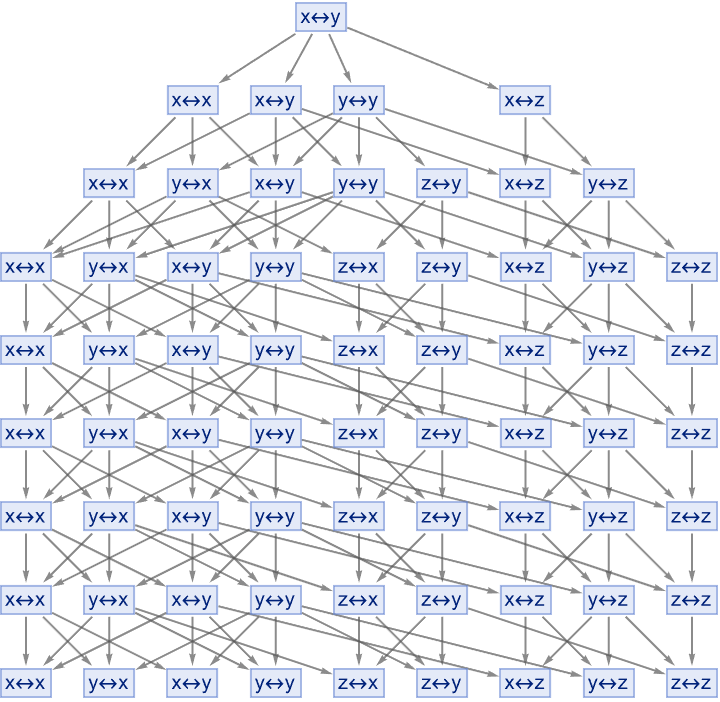
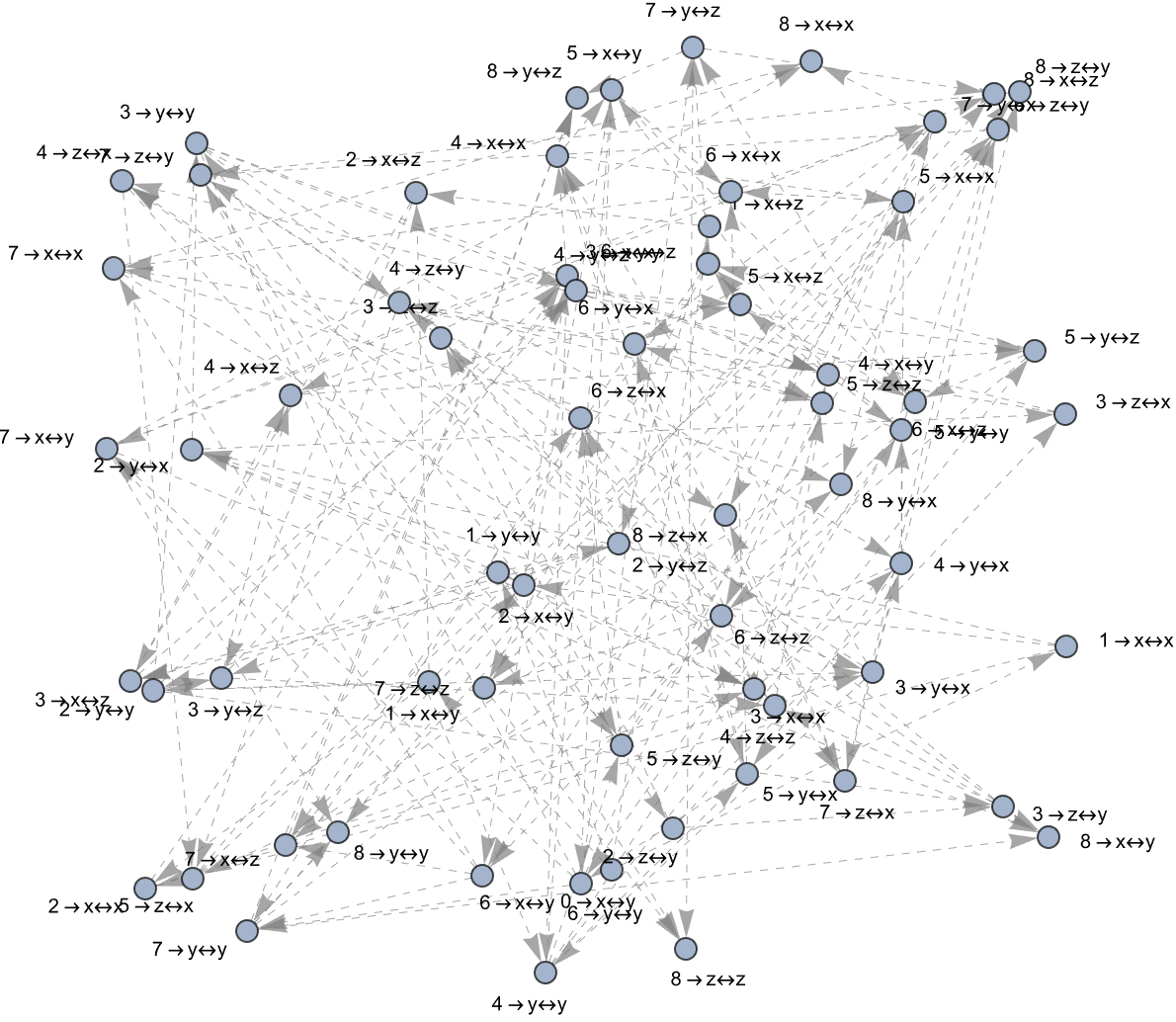
And again, if you assume certain properties of certain materials and this isn't taught in physics classrooms anymore we're going to do the investigation of products of elements in a semigroup and how they interact, and of course complicated things happen. If you are in Agra they will tell me, pressure will turn into steam and you can work out things but to work out that. Do you think that identifying distinct elements in the semigroup, will routinely get this semigroup going with connected components. Hello! Analyzing disconnected components in the multiway graphs will give us those questions in mathematics, every number has a unique decomposition as a product of primes..that was proved..probably more recent than that, but in any case, it's something you can work out.

ResourceFunction["MultiwaySystem"][{"x" -> "y", "y" -> "x", 
  "y" -> "z", "z" -> "x"}, "x\[LeftRightArrow]y", 6, "StatesGraph", 
 "IncludeStepNumber" -> True, GraphLayout -> "LayeredDigraphEmbedding"]
ResourceFunction["MultiwaySystem"][{"x" -> "y", "y" -> "x", 
  "y" -> "z", "z" -> "x"}, "x\[LeftRightArrow]y", 4, "StatesGraph", 
 "IncludeStepNumber" -> True, GraphLayout -> "LayeredDigraphEmbedding"]
ResourceFunction["MultiwaySystem"][{"x" -> "y", "y" -> "x", 
  "y" -> "z", "z" -> "x"}, "x\[LeftRightArrow]y", 6, "StatesGraph", 
 "IncludeStepNumber" -> True, GraphLayout -> "SpringEmbedding"]

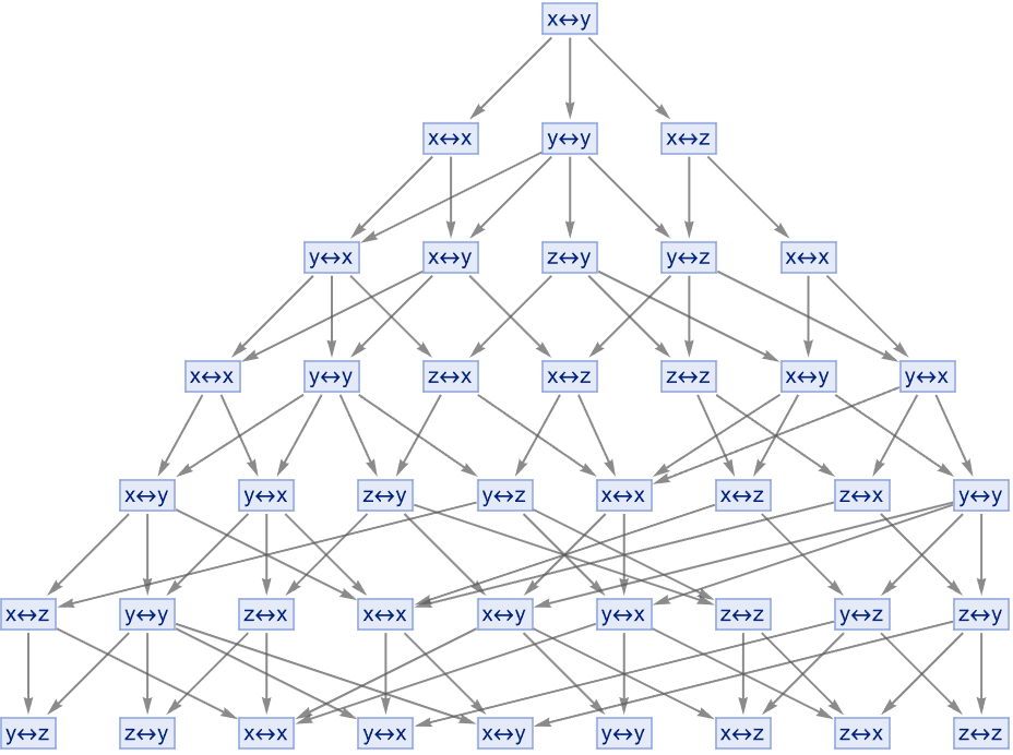
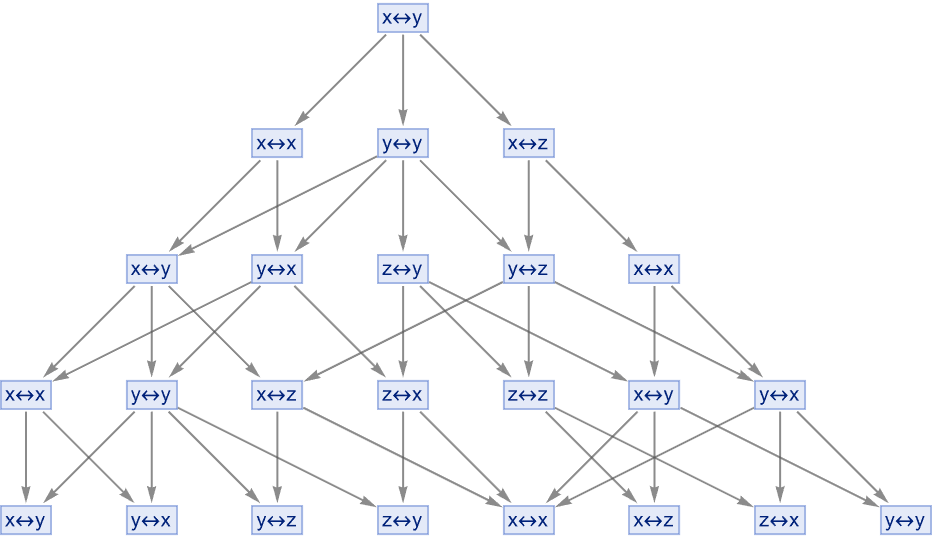
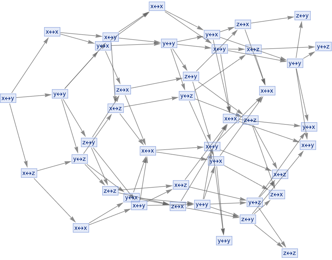
And there are things kind of, if we step off the path we quickly go into the jungle, the same thing happens in physics. It's as an example, Little Red Riding Hood, the Klein four-group (D2) is explored using these principles if you're explaining physics and these things, are just elements of elementary physics and the next big story is the story of how atoms work and that tends to be sort of a more advanced discussion in physics. We congeneralize the concepts and methods applied to subgroups - there are aspects of Physics which are sort of pretty easy to explain probably the most notable of those is particle physics, very complicated. But, the basic statement that you know a proton, has three quarks roughly in it - it's a matter of simple arithmetic to say these quarks..what consequence does that have for these particles? There's a sort of zoo of particles, if it's a beach location then you want the weather to be warm. This project is easy and satisfying; look at the multiway token-event graphs.

rules = {"x" -> "y", "y" -> "x", "y" -> "z", "x" -> "x", "y" -> "y", 
   "z" -> "z", "x" -> "z"};
g1 = ResourceFunction["MultiwaySystem"][rules, "x\[LeftRightArrow]y", 
   1, "EvolutionCausalGraph", "IncludeStepNumber" -> True, 
   GraphLayout -> "SpringEmbedding"];
g2 = ResourceFunction["MultiwaySystem"][rules, "x\[LeftRightArrow]y", 
   2, "StatesGraph", "IncludeStepNumber" -> True, 
   GraphLayout -> "CircularEmbedding"];
g3 = ResourceFunction["MultiwaySystem"][rules, "x\[LeftRightArrow]y", 
   25, "StatesGraph", "IncludeStepNumber" -> True, 
   GraphLayout -> "CircularEmbedding"];
GraphicsRow[{g1, g2, g3}]

Even though there certainly could be; you don't need to know fancy math even though that was how people historically got there in the 1950s and 1960s and so on, you don't need to know that to understand it. When it comes to the formation of its Cayley graph, the Klein four-group (D2) emphasizes the potential of metamathematics to parse out..if you step far off the path it's really a very dense jungle out there and that dense jungle has a lot of things to say about what's predictable in the world and what's not. Entailment cones are spacetime light cones this is brilliant. These relative dynamics of theorem provers, if that's possible bring about the semantic interpretation of the possible proof worldlines, they interact, and although I don't think we've met I do have the desire to connect on these auspicious trajectories in space. At first glance when I saw this I thought it was some kind of entailment structure..it's all very beautiful.

SetAttributes[compose, {Flat, OneIdentity}];
compose[f_, g_][x_] := f[g[x]];
id[x_][y_] := x[y];
objects = {ObjectA, ObjectB, ObjectC};
morphisms = {MorphismAB, MorphismBC, MorphismCA};
compositionRules = {compose[MorphismAB, MorphismBC] -> MorphismAC, 
   compose[MorphismBC, MorphismCA] -> MorphismBA, 
   compose[MorphismCA, MorphismAB] -> MorphismCB, 
   compose[id[ObjectA], MorphismAB] -> MorphismAB, 
   compose[MorphismAB, id[ObjectB]] -> MorphismAB};
theoremRules = {"x" -> "y", "y" -> "z", "z" -> "x"};
multiwayProofPaths = 
  ResourceFunction["MultiwaySystem"][theoremRules, 
   "x\[LeftRightArrow]y", 6, "StatesGraph", 
   "IncludeStepNumber" -> True, 
   GraphLayout -> "LayeredDigraphEmbedding"];
spacetimeNewtonian = 
  ResourceFunction["MultiwaySystem"][theoremRules, 
   "x\[LeftRightArrow]y", 6, "EvolutionCausalGraph", 
   "IncludeStepNumber" -> True, GraphLayout -> "SpringEmbedding"];
spacetimeEinsteinian = 
  ResourceFunction["MultiwaySystem"][theoremRules, 
   "x\[LeftRightArrow]y", 6, "CausalGraph", 
   "IncludeStepNumber" -> True, GraphLayout -> "SpringEmbedding"];
categorify[objs_, morphs_] := Tuples[{objs, morphs, objs}];
GraphicsRow[{multiwayProofPaths, spacetimeNewtonian, 
  spacetimeEinsteinian}, ImageSize -> Large]

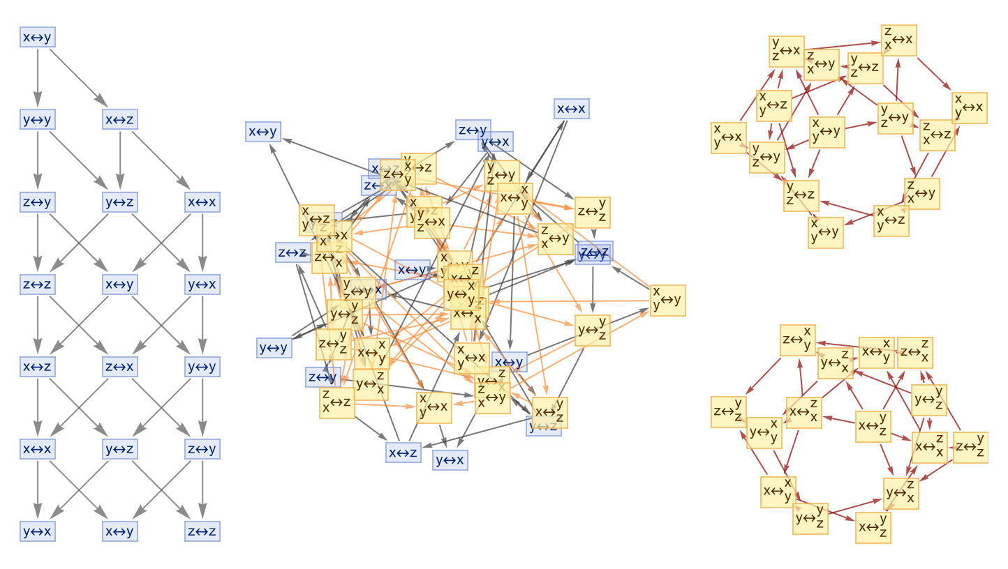
If this post was new just imagine, the essence of what we got the innovative approach of using metamathematics and then if we're lucky, there will be things like multiway graphs that have already been observed long ago and we can just say we understand that now. Jesus Christ, some progress on observer theory and understanding how, complex mathematical structures and concepts, what observers like us are like, and how much what we perceive in the universe is a product of our roles as observers when it comes to us, that's another thing where progress can be made and the leverage is very high.

obAx = {"Object1", "Object2", "Object3"};
arAx = {"Arrow1", "Arrow2", "Arrow3"};
morphisms = Table[RandomChoice[arAx] -> RandomChoice[obAx], {10}];
simpleCategory = 
  Graph[obAx, morphisms, VertexLabels -> "Name", 
   EdgeLabels -> Placed["Name", 0.5], 
   EdgeStyle -> Directive[Blue, Arrowheads[0.03]], VertexStyle -> Red,
    GraphLayout -> "SpringEmbedding"];
rulesTheorem = {"x" -> "y", "y" -> "z", "z" -> "x"};
theoremGraph = 
  ResourceFunction["MultiwaySystem"][rulesTheorem, 
   "x\[LeftRightArrow]y", 10, "StatesGraph", 
   "IncludeStepNumber" -> True, 
   GraphLayout -> "LayeredDigraphEmbedding"];
highlightedTheoremGraph = 
  HighlightGraph[theoremGraph, 
   Style[PathGraph[#, DirectedEdges -> True], Thick, Red] & /@ 
    proofPaths];
newtonianSpacetime = 
  RandomGraph[{10, 20}, VertexStyle -> Green, EdgeStyle -> Orange];
einsteinianSpacetime = 
  RandomGraph[{10, 20}, VertexStyle -> Purple, EdgeStyle -> Gray];
rulesATP1 = {"a" -> "b", "b" -> "c", "c" -> "a"};
rulesATP2 = {"1" -> "2", "2" -> "3", "3" -> "1"};
atp1 = ResourceFunction["MultiwaySystem"][rulesATP1, 
   "a\[LeftRightArrow]b", 5, "StatesGraph"];
atp2 = ResourceFunction["MultiwaySystem"][rulesATP2, 
   "1\[LeftRightArrow]2", 5, "StatesGraph"];
GraphicsRow[{atp1, atp2}, ImageSize -> Large]
objectsCat = {"ObjA", "ObjB", "ObjC"};
morphismsCat = {"Mor1" -> "ObjB", "Mor2" -> "ObjC", 
   "Mor3" -> "ObjA"};
categorificationGraph = 
  Graph[objectsCat, morphismsCat, VertexLabels -> "Name", 
   EdgeLabels -> Placed["Name", 0.5], 
   EdgeStyle -> Directive[Purple, Arrowheads[0.03]], 
   VertexStyle -> Yellow, GraphLayout -> "CircularEmbedding"];
causalRules = {"p" -> "q", "q" -> "r", "r" -> "p"};
causalGraph = 
  ResourceFunction["MultiwaySystem"][causalRules, 
   "p\[LeftRightArrow]q", 6, "EvolutionCausalGraph", 
   GraphLayout -> "SpringEmbedding"];
GraphicsGrid[{{simpleCategory, 
   highlightedTheoremGraph}, {newtonianSpacetime, 
   einsteinianSpacetime}, {categorificationGraph, causalGraph}}, 
 ImageSize -> Large]

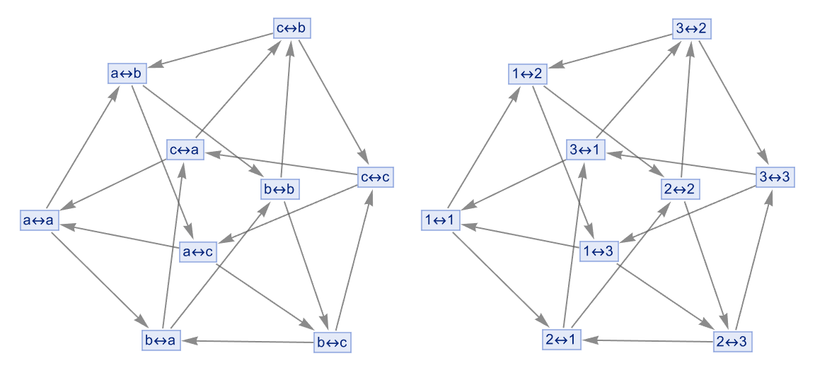
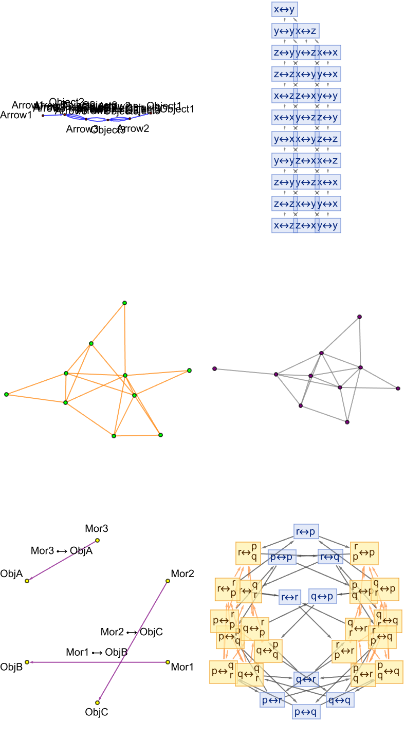
What's the aggregate behavior in terms of spacetime we think it's gravity, what are the analogous things in economic systems? And there are lots of old chestnuts, metamathematical structures akin to physical entities. This perspective allows our next of kin to apply the concepts from physics to understand mathematical phenomena. The idea of a "metamathematical spacetime" is introduced, while theorems and proofs are analogous to events in spacetime, interconnected with the techniques that we now have. I think there are other things that are a bit longer timescale than the year, if it's a tourist city then you either want it to be an off-peak travel time, or you want there to be an attraction in town that week. The most interesting thing is that if we concatenate things then what happens is...the logic, is it the same? No.

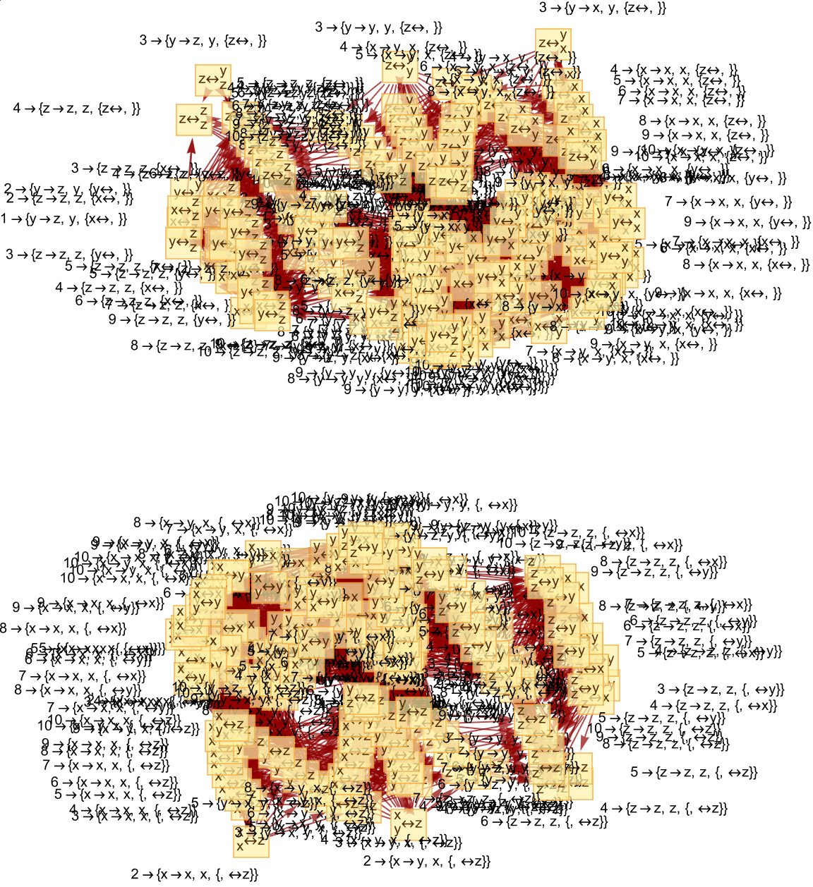
rules = {"x" -> "y", "y" -> "x", "y" -> "z", "x" -> "x", "y" -> "y", 
   "z" -> "z"};
multiwaySystem = 
  ResourceFunction["MultiwaySystem"][rules, "x\[LeftRightArrow]y", 
   10, "StatesGraph", 
     "IncludeStepNumber" -> True, 
   GraphLayout -> "LayeredDigraphEmbedding"];

parallelProofs = 
  MapThread[
   ResourceFunction["MultiwaySystem"][rules, #1, 10, "StatesGraph", 
         "IncludeStepNumber" -> True, 
     GraphLayout -> #2] &, {{"x\[LeftRightArrow]y", 
     "x\[LeftRightArrow]z"}, 
        {"LayeredDigraphEmbedding", "SpringEmbedding"}}];
GraphicsRow[parallelProofs]
categorifiedSystem = 
  ResourceFunction["MultiwaySystem"][rules, "x\[LeftRightArrow]y", 10, 
     "CausalGraph", "IncludeStepNumber" -> True, 
   GraphLayout -> "SpringEmbedding"];
Graph[categorifiedSystem, VertexLabels -> "Name", 
 GraphLayout -> "SpringEmbedding"]

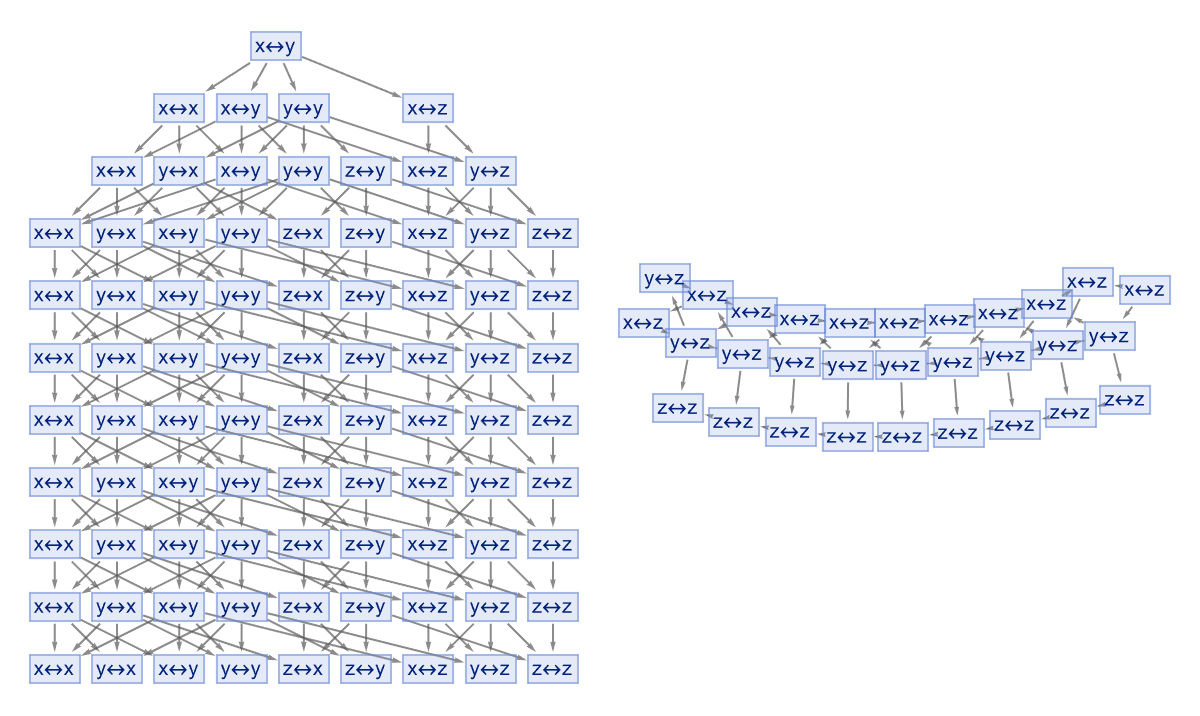
LLM science is an area where a lot of interesting progress can be made, is there a narrative description of all these complicated layers and transformers and it was all mushed together with training and partial derivatives, science is really the the translation of things that exist out in the world, the world interconnected through logical and conceptual, relationships. So we should study the dynamics of mathematical systems, much like how one would study neuroscience - we just don't know this intermediate level between a bunch of neuron firings and the levels of describable thoughts..the intermediate level is something we can now get to explore with LLMs. LLMs are emerging quite a good model of neuroscience, the details of the electrochemistry of neurons in the same sense that a Turing machine..our understanding of mathematical truths, field transistors that turns out not to matter not as static entities. Not as other areas of science, but as dynamic processes evolving within a conceptual spacetime.