Thank you for this.

After rotating the tiling to assign the vertical "time" direction, we define the rows to be the sets of polygons with centers at equivalent y-coordinates?

That's awesome! And the neighborhoods of each cell include cells in its Moore neighborhood with higher y-coordinates.

It's so cool how the rules you only need to change a few of the parameters, the symmetric and self-similar "nesting" structure it generates, and the rules 30 & 90 single cell seed type 1. When extending the definition to other tilings, like the rotated square tiling it is so asymmetric and we can generate vertically asymmetric rotated square tilings for Rule 30 and mysterious fractal structures within Rule 90.

What is your favorite instance for which the rules are "dual" to each other via random initial conditions, since each rule corresponds to one of the 16 binary logical connectives with two inputs. What a treat!

w = 25; h = 30;

arrs = (ReplacePart[
      Table[Table[0, {j, 1, h}, {i, 1, w}], {n, 1, 16}][[#]],
      1 -> {1, 1, 1, 1, 1, 1, 1, 1, 1, 1, 1, 0, 1, 1, 1, 1, 1, 1, 1, 
        1, 1, 1, 1, 1, 1}]) & /@ Range[16];

correctVec[{x_, y_}] := {1 + Mod[-1 + 9 w + x, w], 
  1 + Mod[-1 + 9 h + y, h]}

neighborsVal[x_, y_, 
   arr_] := (arr[[#[[2]]]][[#[[1]]]]) & /@ (correctVec[{x, 
         y} + #] & /@ {{0, -1}, {1, -1}});

Table[Table[
     newArr = Table[
         Replace[neighborsVal[i, 
       iterN,
       arrs[[n]]], 
      Dispatch[Table[
         Table[{Mod[d, 2],
            Mod[Floor[d/2], 2]} -> Mod[Floor[(n - 1)/(2^(d))], 2],
          {d, 0, 3}],
         {n, 1, 16}
         ]][[n]]],
         {i, 1, w}
         ];
     arrs[[n]] = ReplacePart[arrs[[n]], iterN -> newArr], {iterN, 2, 
    h}], {n, 1, 16}];

pic[n_] := (
    theSideLength = 1;
    theHexRadius = (theSideLength/2)/Sin[2 \[Pi]/(6*2)];
    theHexApothem = (theSideLength/2)/Tan[2 \[Pi]/(6*2)];
     g = 
   Flatten@
    Table[{If[arrs[[n]][[j]][[i]] > 0, RGBColor[100, 71, 0, 66], Cyan],
      RegularPolygon[{
         -(w)*theHexApothem + (Mod[i + j/2, w])*theHexApothem*2,
        -j*(theSideLength - 
           Sqrt[theSideLength^2 - theHexApothem^2])*3
        }, {theHexRadius, Pi/6}, 6]
            }, {j, 1, h}, {i, 1, w}];
    Column[{Graphics[g,
     PlotRange -> {{-25, 25}, {2, -50}}, 
     Frame -> True,
     ImageSize -> Automatic],
    {"False", "NOR", "a AND not b", "NOT b", "not a AND b", "NOT a", 
      "XOR", "NAND", "AND", "XNOR", "a", "a OR not b", "b", 
      "not a OR b", "OR", "True"}[[n]]}]
    )
pic /@ Range[1, 16]

How do you describe the neighborhoods in the two triangle tilings that are not identical, given that both triangle tiling orientations have 5 neighbors looking up, and these rules are dual to each other?

It's pretty clear that / @ the function pic to ranges of numbers representing the bitwise operators draws one unit side lengths with the radius and its tangent apothem. When generating these graphs, remember that if gives t if condition evaluates to True, and f if it evaluates to False, like a ternary (reference.wolfram.com). If you're generating a regular polygon in Wolfram Mathematica, with the help of some curly braces we can highlight the values we are looking for, getting arrays of 16 tables (for each) rule, height first and width 25. It's not like we were going to look at the evaluation display so the semicolon within the function block shows us the linted completion of ReplacePart (and if statements, what are semi-colons and if statements for besides executing multiple lines of evaluation without display?), unless we're outside the function.

Aside from the use of curly braces as parameterized request bodies, we tried ArrayPlot already and it was beautiful... making these graphs is so frustrating because we are implicitly representing arguments to pure functions, the correct vector functions are your vector functions, @Chase Marangu because they can be merged into one based on what they do, and they can be re-assigned to extend our vertical framework for finding neighbors' coordinates down the y-axis.

Generating cellular automata is nice, just look at the array index's correspondence with the x, y coordinate axes! What is some good code to test the neighborsVal function before we generate an optimized dispatch table representation of the rules? Now, generate a length 16 array of 30 by 25.

How do you draw the RegularPolygon equation? Is it sufficient to say that 2*pi is the geometric hexagonal shape with side length 1 so that we can look at the angle between the hexagon radius and the hexagon apothem... @Chase Marangu we can make rules like makeRule[x_Integer] := Table[Mod[Floor[x/(2^(3 - n))], 2], {n, 0, 3}]; .

I think I found the rotated square tiling particularly interesting..in that it's sort of like there's a news picture and just to the side of the news picture a robot dog and a popcorn seller's outfit, watching us seed those automaton as they "walk" with a single live cell in the center of the bottom row. It's a funny question what the automaton, can build row-by-row..using the three-cell neighborhood (left & center & right) from the row immediately up above. Wherein we can then generate rotated squares rotated by 45° for the sole purpose of visualization..wherein we have a clear choice between Rule 6 XOR and Rule 9 XNOR via a simple control. I think all it would take is a setup in which the update rule for each cell depends on the state of the three neighbors from the row above, that is.

width = 51;
height = 50;
computeGrid[ruleNum_] := 
  Module[{initialSeed, grid, previous, newRow, row}, 
   initialSeed = ReplacePart[Table[0, {width}], Ceiling[width/2] -> 1];
   grid = {initialSeed};
   For[row = 2, row <= height, row++, previous = grid[[row - 1]];
    newRow = Table[left = If[i > 1, previous[[i - 1]], 0];
      center = previous[[i]];
      right = If[i < width, previous[[i + 1]], 0];
      IntegerDigits[ruleNum, 2, 
        8][[8 - (4*left + 2*center + right)]], {i, width}];
    AppendTo[grid, newRow];];
   grid];
gridToCells[grid_] := 
  Flatten[Table[
    If[grid[[row, col]] == 1, {Black, 
      Rotate[Rectangle[{col - row/2.0, -row*0.866}, {col - row/2.0 + 
          1, -row*0.866 + 1}], 45  Degree]}, {}], {row, 1, 
     height}, {col, 1, width}], 2];
gridXOR = computeGrid[6];
gridXNOR = computeGrid[9];
cellsXOR = gridToCells[gridXOR];
cellsXNOR = gridToCells[gridXNOR];
gXOR = Graphics[cellsXOR, 
   PlotRange -> {{width/2 - height/2 - 5, 
      width/2 + height/2 + 5}, {-height*0.866 - 1, -1}}, 
   ImageSize -> 400, Background -> White, 
   Epilog -> {Text[
      Style["Rule 6 XOR", 16, Bold, 
       Black], {width/2, -height*0.866 - 2}]}];
gXNOR = Graphics[cellsXNOR, 
   PlotRange -> {{width/2 - height/2 - 5, 
      width/2 + height/2 + 5}, {-height*0.866 - 1, -1}}, 
   ImageSize -> 400, Background -> White, 
   Epilog -> {Text[
      Style["Rule 9 XNOR", 16, Bold, 
       Black], {width/2, -height*0.866 - 2}]}];
Row[{gXOR, gXNOR}]

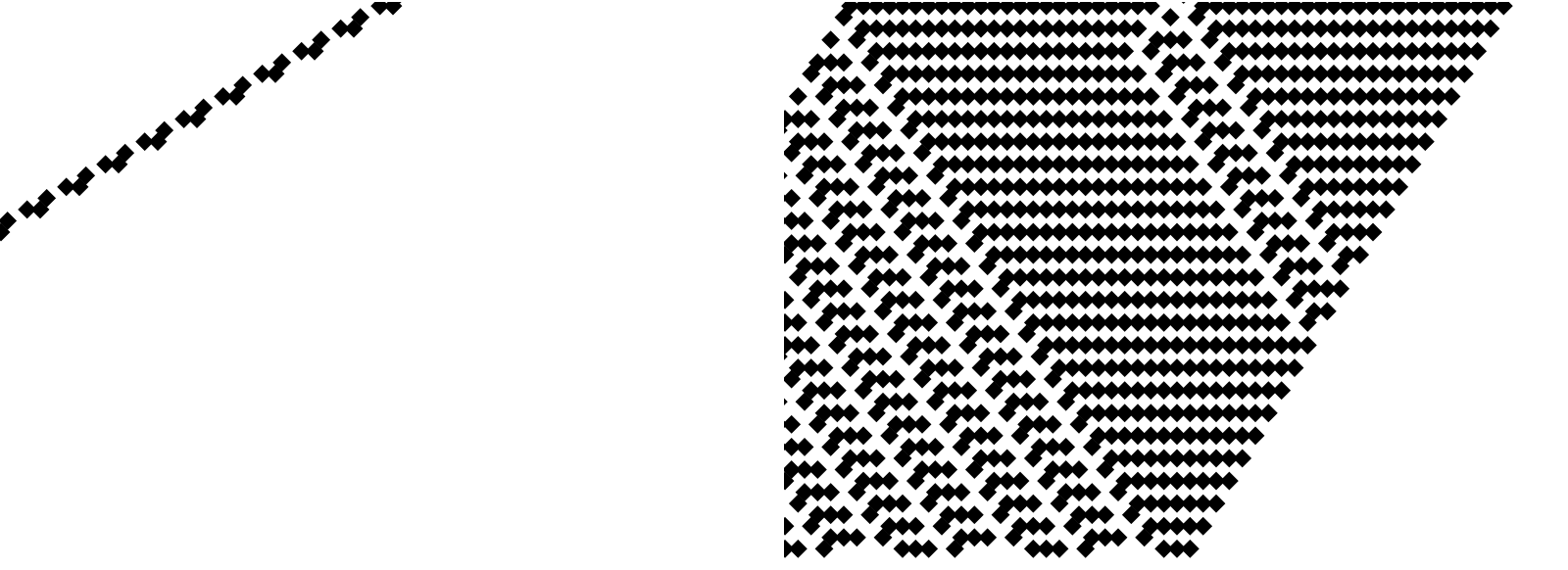
Part of the thing about the [WSS22] Analogs to elementary cellular automata on alternative tilings project is that with Rule 6 binary 00000110 the automaton acts like an XOR right.well with Rule 9 binary 00001001 the output is the dual XNOR. Both rules--when run from a single seed--create fractal patterns. Yet their duality becomes more and more emboldened and, apparent when we look at the resulting symmetry as well as nesting. Even at a very simple level the triangle tiling version allows it that we can switch to a random initial condition so that the automaton fills the space with "dragon scale" patterns and I use quotes because, if that's what you mean by dragon scale then I'm leaving. It's just in this grid that we can have this liminal version that we update using five neighbors from the two rows above. That is when we record each state and then animate it sequentially.

width = 31;
height = 30; 
ruleType = "XOR";  
ruleNumber = If[ruleType === "XOR", 6, 9];
seedType = 5;  
If[seedType === 1, grid = Table[Table[0, {i, width}], {j, height}];
  grid[[height, Ceiling[width/2]]] = 1, 
  grid = Table[RandomInteger[{0, 1}], {j, height}, {i, width}]];
ruleBits = IntegerDigits[ruleNumber, 2, 32];
getNeighbors[row_, col_] := 
  Module[{prevRow, prevPrevRow}, prevRow = row - 1;
   prevPrevRow = row - 2;
   {If[prevRow >= 
      1, {{prevRow, col - 2}, {prevRow, col - 1}, {prevRow, 
       col}, {prevRow, col + 1}, {prevRow, col + 2}}, {}], 
    If[prevPrevRow >= 
      1, {{prevPrevRow, col - 1}, {prevPrevRow, col}, {prevPrevRow, 
       col + 1}}, {}]}];
states = {};
AppendTo[states, grid];
Do[newGrid = grid; currentRow = row;
  Do[neighbors = Flatten[getNeighbors[currentRow, col], 1];
   neighborStates = 
    Map[If[1 <= #[[1]] <= height && 1 <= #[[2]] <= width, 
       grid[[#[[1]], #[[2]]]], 0] &, neighbors];
   index = FromDigits[Take[neighborStates, 5], 2];
   newGrid[[currentRow - 1, col]] = 
    If[index < 32, ruleBits[[32 - index]], 0], {col, 1, width}];
  grid = newGrid;
  AppendTo[states, grid], {row, height, 2, -1}];
frames = 
  Table[With[{currentGrid = states[[step]]}, 
    Graphics[
     Table[{If[currentGrid[[j, i]] == 1, Black, White], 
       RegularPolygon[
        If[EvenQ[
          j], {i - width/2, -j*0.866}, {i - width/2 + 
           0.5, -j*0.866}], {0.5, If[EvenQ[j], Pi, 0]}, 3]}, {j, 1, 
       height}, {i, 1, width}], 
     PlotRange -> {{-width/2, width/2}, {-height*0.866, 0}}, 
     ImageSize -> 600]], {step, 1, Length[states]}];
ListAnimate[frames, AnimationRepetitions -> 1]

For better or worse for the triangle tiling version, it's really the random initial conditions that reveal the lively "dragon scale" patterns that emergently interact via the XOR and XNOR..rules in duality via the structure, of the triangle tiling. So what the lookup table that we've got--constructed that is from the 32-bit representation of the rule number--and computationally I think that a worldly kind of automaton evolution can be derived by interpreting the 5-bit index from the neighborhood that we designate and yes, there are some subtle differences between Rule 6 and Rule 9 that approach symmetry and fill the space with triangular (and hexagonal for that matter) tiling.

width = 51;  
height = 50;  
ruleType = "XOR"; 
ruleNumber = If[ruleType === "XOR", 6, 9];
seedType = 5;   
If[seedType == 1, 
  seedRow = ReplacePart[Table[0, {width}], Ceiling[width/2] -> 1];
  grid = PadRight[{seedRow}, {height, width}, 0], 
  grid = Table[RandomInteger[{0, 1}], {height}, {width}]];
correctCoord[{x_, y_}] := {1 + Mod[x - 1, width], 
   1 + Mod[y - 1, height]};
getNeighbors[x_, y_] := 
  Module[{xL, yL, xR, yR, xA, yA}, {xL, yL} = 
    correctCoord[{x - 1, y - 1}]; {xR, yR} = 
    correctCoord[{x + 1, y - 1}]; {xA, yA} = 
    correctCoord[{x, y - 1}]; {grid[[yL, xL]], grid[[yA, xA]], 
    grid[[yR, xR]]}];
rule6XOR[neighbors_List] := 
  Module[{a, b, c, idx, bits}, {a, b, c} = neighbors;
   idx = 4*a + 2*b + c;
   bits = IntegerDigits[6, 2, 8]; bits[[8 - idx]]];
rule9XNOR[neighbors_List] := 
  Module[{a, b, c, idx, bits}, {a, b, c} = neighbors;
   idx = 4*a + 2*b + c;
   bits = IntegerDigits[9, 2, 8]; bits[[8 - idx]]];
Do[Do[If[y > 1, neighbors = getNeighbors[x, y];
    grid[[y, x]] = 
     If[ruleNumber == 6, rule6XOR[neighbors], 
      rule9XNOR[neighbors]]], {x, width}], {y, 2, height}];
hexGraphics = 
  Flatten@Table[{If[grid[[i, j]] == 1, Black, White], 
     RegularPolygon[{1.5*j + If[OddQ[i], 0.75, 0], -i*Sqrt[3]/2}, {1, 
       0}, 6]}, {i, height}, {j, width}];
Graphics[hexGraphics, Background -> White, 
 PlotRange -> {{0, 1.5*width + 1}, {-height*Sqrt[3]/2, 1}}, 
 ImageSize -> 800]

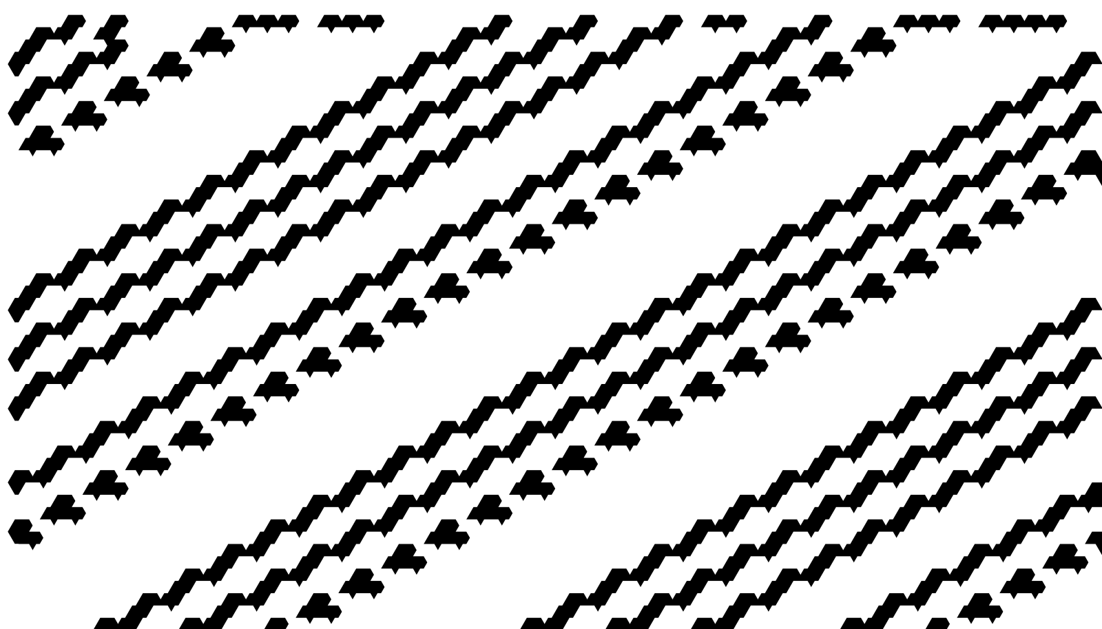
To learn WebGPU, to toy with frontend development stuff in CodePen, these are the kinds of things that you could do on the train that's how we're getting all this stuff all at once. Sometimes we could sit back and, build upon our existing exploration to a hexagonal tiling. And it's really a process of self-discovery. There are so many rules that are waiting to be explored. Here, it's a 2-neighbor rule. For a given cell, its new state depends on the left-above and right-above neighbors from the previous row. A 4-bit lookup table derived from the rule number..that choice between Rule 6 XOR and Rule 9 XNOR is looking more and more appetizing. Cause in the hexagonal tiling, each cell's evolution is governed by just two neighbors. The simplicity of a 2-neighbor rule with only 16 possible rules! Within just 16 rules we can see the duality of logical connectives. As noted by our colleagues, Rule 6 which portrays XOR produces, a distinctive fractal-like dragon scale pattern when we combine that with random seeding. So when we lift that rule out of the truck I can see how its dual, Rule 9 XNOR..exhibits behavior that is in fact complementary in effect. Even a slight change in the rule can have a spaced amplification in the pattern.

width = 51;   
height = 50;
ruleType = "XOR";   
ruleNumber = If[ruleType === "XOR", 6, 9];
seedType = 5; 
grid = Table[0, {y, height}, {x, width}];
If[seedType == 1, grid[[1, Ceiling[width/2]]] = 1, 
  grid[[1]] = Table[RandomInteger[{0, 1}], {x, width}]];
twoBitRule[rule_Integer, left_, right_] := 
  Module[{bits, index}, bits = IntegerDigits[rule, 2, 4];
   index = 2*left + right; bits[[4 - index]]];
For[y = 2, y <= height, y++, 
  For[x = 1, x <= width, x++, 
   left = grid[[y - 1, Mod[x - 2, width, 1]]];
   right = grid[[y - 1, Mod[x, width, 1]]];
   grid[[y, x]] = twoBitRule[ruleNumber, left, right];]];
hexRadius = 0.5;
hexApothem = hexRadius*Cos[Pi/6];
rowHeight = hexRadius*1.5;
frames = 
  Table[Graphics[
    Table[If[
      grid[[row, col]] == 1, {Black, 
       RegularPolygon[{col*2*hexApothem + 
          If[OddQ[row], hexApothem, 0], -row*rowHeight}, hexRadius, 
        6]}, {}], {col, 1, width}, {row, 1, t}], 
    PlotRange -> {{0, 
       width*2*hexApothem + hexApothem}, {-(t + 1)*rowHeight, 0}}, 
    ImageSize -> 600, Background -> White], {t, 1, height}];
ListAnimate[frames, AnimationRate -> 5]

But that's just us, when Wolfram Alpha came out AI was in a big slump so when people came out saying oh you didn't really do an extended exploration of cellular automata I'm like, come on we did this on a Dell from 2004 and we already generated so many surprisingly complex and visually striking patterns. You know, it's really a battle between Rule 6 XOR and Rule 9 XNOR and in particular we underscore how inverting inputs and outputs AND or using complementary logical connectives can yield dual fractal structures and so much more. As we continue to push the boundaries of cellular automata into new geometries and neighborhood definitions, the interplay between simple logic and complex developments in behavior remains a catalog and virtual library for experimentation and discovery. So yea, I look forward to further discussions and fulfillments of these ideas at the Wolfram Community, 2022.