Building on your setup, we can turn AdinkraManualGraph3D[] into an interactive exploration tool by adding controls that let you slide through different vertex-weight schemes or edge-color mappings on the fly, and by the way, the radial coordinate r, toggles, to flip vertex colors by sign. And we have a dropdown to switch between multiple colors associations (say, alternative palettes for Green/Purple/Orange/Red). It's pretty important to ask questions like why we do the things we do, but we shouldn't be asking those questions. Those questions, won't have a sequel. Most of our Mathematica, we learned it by drinking through the hose of academia, the ethos of Wolfram's multiway systems--it's all very wrong but, that's the way why we keep doing these Adinkras. So speaking of "ethos", this girl I know (don't know her name it starts with a D or an L like Leah..but anyway) was giggling about all this, to me explaining all the scientific articles they're written in Latin and Greek. And you don't wanna know what I said but it was the inevitable, how do two and two go together? You liar! So instead, we have this series of interactions, which progressively lead us to the invitation: to live inside the mathematics rather than merely view it--and that, switch between observer and system lies at the heart of the Wolfram-Physics philosophy. So how about that? I love languages but there's nothing like some fresh, Mathematica landscape that got me dreaming in Wolfram Language. I was even dreaming it was a full, complete algebraic structure I was completely fulfilled. I was totally smitten with the kinematic shifts, in the 3-dimensional graph or matrix plots which become a thought experiment. In how physical symmetries might flex, under different "observational frames," reinforcing that an adinkra is as much about the relationships it encodes as the "decisions we make", as it is about the choice of perspective you bring to it. And that's why we need the live and interaction dimension of the adinkra. And I think this might be able to explain some of it.

ClearAll[vertices, vertexWeights, edges, edgeWeights, colors];
vertices = {A, B, F, G, \[Psi]1, \[Psi]2, \[Psi]3, \[Psi]4};
vertexWeights = {1, 1, 3, 3, -2, -2, -2, -2};
edges = {A -> \[Psi]2, B -> \[Psi]4, \[Psi]3 -> F, \[Psi]1 -> G, 
   A -> \[Psi]4, B -> \[Psi]2, \[Psi]1 -> F, \[Psi]3 -> G, 
   A -> \[Psi]1, B -> \[Psi]3, \[Psi]4 -> F, \[Psi]2 -> G, 
   A -> \[Psi]3, B -> \[Psi]1, \[Psi]2 -> F, \[Psi]4 -> G};
edgeWeights = {2, -1, 4, 3, 4, -3, -2, -1, 1, 2, -3, 4, 3, 4, 1, -2};
colors = <|1 -> Green, 2 -> Purple, 3 -> Orange, 4 -> Red|>;
coords = 
  AssociationThread[vertices, 
   Module[{n = Length[vertices], r = 2}, 
    Table[With[{\[Theta] = 2 Pi (i - 1)/n}, {r Cos[\[Theta]], 
       r Sin[\[Theta]], 1.5 vertexWeights[[i]]}], {i, n}]]];
AdinkraManualGraph3D[] := 
  Module[{nodes, tubes, labels}, 
   nodes = Table[{If[vertexWeights[[i]] > 0, White, Black], 
      Specularity[White, 10], 
      Sphere[coords[vertices[[i]]], 0.12]}, {i, Length[vertices]}];
   tubes = 
    Table[{colors[Abs[edgeWeights[[i]]]], Specularity[White, 5], 
      Tube[{coords[edges[[i, 1]]], coords[edges[[i, 2]]]}, 
       0.035]}, {i, Length[edges]}];
   labels = 
    Table[Text[Style[ToString[vertices[[i]]], 16, Bold, White], 
      coords[vertices[[i]]], {0, 0}], {i, Length[vertices]}];
   Graphics3D[{tubes, nodes, labels}, Boxed -> False, 
    Lighting -> "Neutral", ImageSize -> 400]];
LMatrices = {{{1, 0, 0, 0}, {0, 0, 0, -1}, {0, 1, 0, 0}, {0, 0, -1, 
     0}}, {{0, 1, 0, 0}, {0, 0, 1, 0}, {-1, 0, 0, 0}, {0, 0, 
     0, -1}}, {{0, 0, 1, 0}, {0, -1, 0, 0}, {0, 0, 0, -1}, {1, 0, 0, 
     0}}, {{0, 0, 0, 1}, {1, 0, 0, 0}, {0, 0, 1, 0}, {0, 1, 0, 0}}};
VisualizeMatrix[m_] := 
  ArrayPlot[m, ColorRules -> {1 -> Green, -1 -> Red, 0 -> White}, 
   Frame -> True, FrameTicks -> All, 
   PlotLabel -> Style["Adinkra Matrix Representation", 12, Bold]];
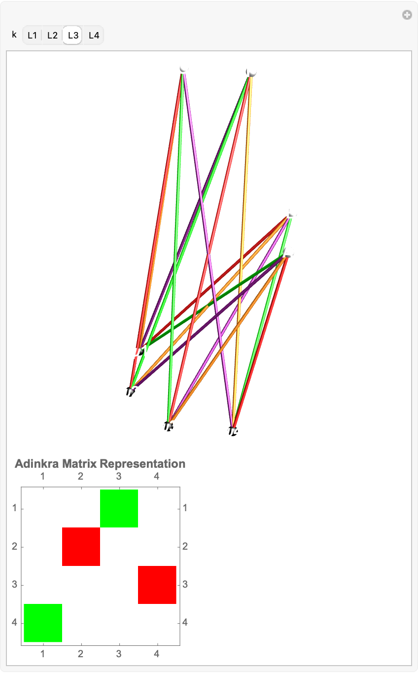
Manipulate[
 Column[{AdinkraManualGraph3D[], VisualizeMatrix[LMatrices[[k]]]}, 
  Spacing -> 20], {k, 1, 4, 1, 
  SetterBar[#, {1 -> "L1", 2 -> "L2", 3 -> "L3", 4 -> "L4"}] &}, 
 ControlPlacement -> Top, FrameMargins -> 0]

And golly gee I think the Mathematica 14.0 has done it again. But, this is a "very brief" article and I think that the Adinkra, if I look it up this is what I get:

Next question. It's pretty clear that we can cluster vertices but "how low can those vertices go" is the real question. I have this layout that layers vertices based on their weights and then radially distributes each group at a radius scaled by the magnitude of its weight. Positive-weight nodes float above the plane, negatives below, so bosons and fermions occupy distinct strata, and heavier vertices sit farther out. The reader, edges pick up the same color-and-dash semantics as before but now trace between these "tiered" rings. The result is a 3-dimensional adinkra whose geometry directly projects both the algebraic "level" of each field (via height and ring radius) and sign/the magnitude of its connections, making the supersymmetry structure legible in space.

vertices = {"A", "B", "F", "G", "psi1", "psi2", "psi3", "psi4"};
vertexWeights = {1, 1, 3, 3, -2, -2, -2, -2};
edges = {"A" -> "psi2", "B" -> "psi4", "psi3" -> "F", "psi1" -> "G", 
   "A" -> "psi4", "B" -> "psi2", "psi1" -> "F", "psi3" -> "G", 
   "A" -> "psi1", "B" -> "psi3", "psi4" -> "F", "psi2" -> "G", 
   "A" -> "psi3", "B" -> "psi1", "psi2" -> "F", "psi4" -> "G"};
edgeWeights = {2, -1, 4, 3, 4, -3, -2, -1, 1, 2, -3, 4, 3, 4, 1, -2};
colorScheme = <|1 -> Green, 2 -> Purple, 3 -> Orange, 4 -> Red|>;
AdinkraCoords[vs_, ws_] := 
  Module[{groups, h = 2, r0 = 1, coordRules}, 
   groups = GatherBy[Transpose[{vs, ws}], Last];
   coordRules = 
    Flatten@Table[
      With[{w = grp[[1, 2]], 
        n = Length[grp], \[Theta] = 2 \[Pi]/Length[grp], 
        r = r0 (1 + Abs[grp[[1, 2]]]/5)}, 
       Table[grp[[i, 1]] -> {r Cos[(i - 1) \[Theta]], 
          r Sin[(i - 1) \[Theta]], Sign[w] (Abs[w] + h)}, {i, 
         Length[grp]}]], {grp, groups}];
   coordRules];
coords = AdinkraCoords[vertices, vertexWeights];
pos[k_String] := (k /. coords);
vertexObjects = 
  Table[{If[vertexWeights[[i]] > 0, White, GrayLevel[.3]], 
    Sphere[pos[vertices[[i]]], .15], 
    Text[Style[vertices[[i]], White, Bold, 14], 
     pos[vertices[[i]]] + {0, 0, .25}]}, {i, Length[vertices]}];
edgeObjects = 
  Table[Module[{p1, p2, w, col, style}, p1 = pos[edges[[i, 1]]];
    p2 = pos[edges[[i, 2]]];
    w = edgeWeights[[i]];
    col = colorScheme[Abs[w]];
    style = 
     If[w < 0, {col, Dashed, Thickness[.015]}, {col, Thickness[.015]}];
    {style, Tube[{p1, p2}, 0.03]}], {i, Length[edges]}];
Graphics3D[{Lighting -> "Neutral", vertexObjects, edgeObjects}, 
 Boxed -> False, ImageSize -> 200, ViewPoint -> {3, -2, 1.5}]

And so we need more fillers..of course I would not buy any of these arrangements and that's why we need all these arrangements, because we've "already started the brainwashing process"..but just kidding. I always thought of the living topography of the Ruliad as radiating concentric rings whose radii grow with the vertex weight and lifting positive-weight nodes above (while sinking negatives below). It's too much of a coincidence, to not be the supersymmetry algebra; heavy multiplets fan out to the periphery, and every edge becomes a bridge whose color and pattern directly trace the strength and sign of that algebraic relation.

AdinkraVertexCoordinates3D[vertices_List, vertexweights_List] := 
 Module[{groups, coords = {}, z, count, angles, x, y, groupIndices}, 
  groups = 
   GatherBy[Range[Length[vertices]], Norm[vertexweights[[#]]] &];
  Do[groupIndices = groups[[i]];
   z = Norm[vertexweights[[groupIndices[[1]]]]];
   count = Length[groupIndices];
   angles = Range[0, 2 Pi - 2 Pi/count, 2 Pi/count];
   x = Cos[angles];
   y = Sin[angles];
   coordGroup = Transpose[{x, y, ConstantArray[z, count]}];
   coords = 
    Join[coords, Thread[vertices[[groupIndices]] -> coordGroup]];, {i,
     Length[groups]}];
  coords]
AdinkraGraph3D[vertices_List, vertexweights_List, edges_List, 
  edgeweights_List, colors_Association] := 
 Graph3D[vertices, 
  Style[edges[[#]], {colors[Abs[edgeweights[[#]]]], 
      If[Sign[edgeweights[[#]]] < 0, Dashed, Nothing], Thick}] & /@ 
   Range[Length[edges]], 
  VertexStyle -> 
   Table[vertices[[i]] -> 
     Directive[EdgeForm[Black], 
      If[Sign[vertexweights[[i]]] > 0, White, Black], 
      Specularity[White, 30]], {i, Length[vertices]}], 
  VertexSize -> Large, 
  VertexCoordinates -> 
   AdinkraVertexCoordinates3D[vertices, vertexweights], 
  ImageSize -> Full, Boxed -> False, 
  EdgeLabels -> Placed["EdgeWeight", 0.5], 
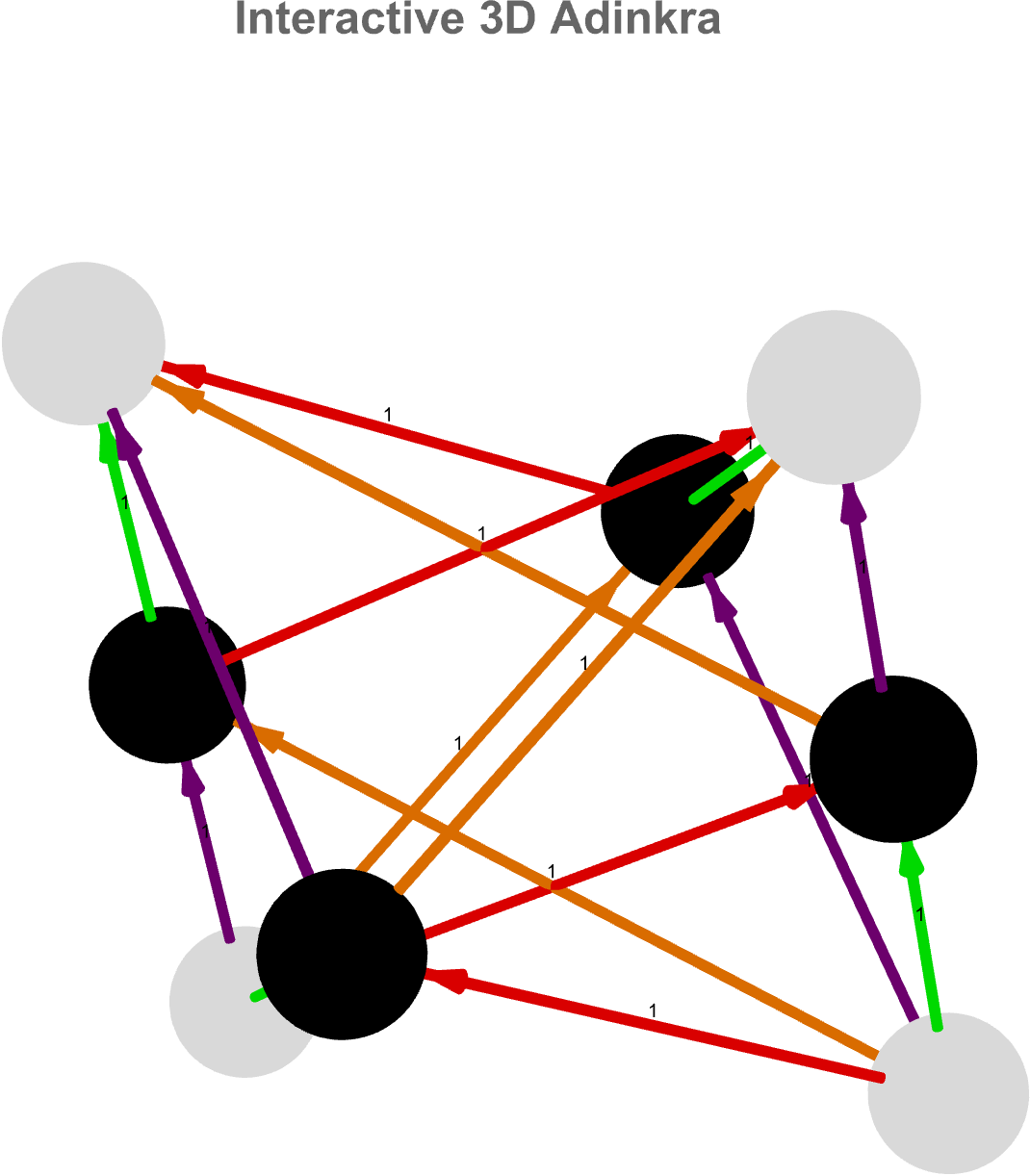
  PlotLabel -> 
   Style["Interactive 3D Adinkra", Bold, 24, FontFamily -> "Arial"], 
  ViewPoint -> {1.5, -2.5, 1.8}, ViewVertical -> {0.1, 0.2, 1.0}, 
  Lighting -> {{"Ambient", LightGray}}, 
  PlotRangePadding -> Scaled[0.2], PerformanceGoal -> "Quality"]
vertices = {A, B, F, G, Subscript[\[CapitalPsi], 1], 
   Subscript[\[CapitalPsi], 2], Subscript[\[CapitalPsi], 3], 
   Subscript[\[CapitalPsi], 4]};
vertexweights = {1, 1, 3, 3, -2, -2, -2, -2};
edges = {A -> Subscript[\[CapitalPsi], 2], 
   B -> Subscript[\[CapitalPsi], 4], Subscript[\[CapitalPsi], 3] -> F,
    Subscript[\[CapitalPsi], 1] -> G, 
   A -> Subscript[\[CapitalPsi], 4], B -> Subscript[\[CapitalPsi], 2],
    Subscript[\[CapitalPsi], 1] -> F, 
   Subscript[\[CapitalPsi], 3] -> G, A -> Subscript[\[CapitalPsi], 1],
    B -> Subscript[\[CapitalPsi], 3], 
   Subscript[\[CapitalPsi], 4] -> F, Subscript[\[CapitalPsi], 2] -> G,
    A -> Subscript[\[CapitalPsi], 3], 
   B -> Subscript[\[CapitalPsi], 1], Subscript[\[CapitalPsi], 2] -> F,
    Subscript[\[CapitalPsi], 4] -> G};
edgeweights = {2, -1, 4, 3, 4, -3, -2, -1, 1, 2, -3, 4, 3, 4, 1, -2};
colors = <|1 -> Green, 2 -> Purple, 3 -> Orange, 4 -> Red|>;
AdinkraGraph3D[vertices, vertexweights, edges, edgeweights, colors]

These mathematical objects representing supersymmetric particles, in physics oh my goodness! If there's one thing I do remember it's how philosophically, this layered, radial design crystallizes the notion that an adinkra isn't just a static encoding of equations but a spatial manifestation of how different fields "orbit" one another under supersymmetric, reminding us that algebraic structures are, at heart, geometric processes unfolding through levels of abstraction.

vertices = {A, B, F, G, Subscript[\[CapitalPsi], 1], 
   Subscript[\[CapitalPsi], 2], Subscript[\[CapitalPsi], 3], 
   Subscript[\[CapitalPsi], 4]};
vertexweights = {1, 1, 3, 3, -2, -2, -2, -2};
edges = {A -> Subscript[\[CapitalPsi], 2], 
   B -> Subscript[\[CapitalPsi], 4], Subscript[\[CapitalPsi], 3] -> F,
    Subscript[\[CapitalPsi], 1] -> G, 
   A -> Subscript[\[CapitalPsi], 4], B -> Subscript[\[CapitalPsi], 2],
    Subscript[\[CapitalPsi], 1] -> F, 
   Subscript[\[CapitalPsi], 3] -> G, A -> Subscript[\[CapitalPsi], 1],
    B -> Subscript[\[CapitalPsi], 3], 
   Subscript[\[CapitalPsi], 4] -> F, Subscript[\[CapitalPsi], 2] -> G,
    A -> Subscript[\[CapitalPsi], 3], 
   B -> Subscript[\[CapitalPsi], 1], Subscript[\[CapitalPsi], 2] -> F,
    Subscript[\[CapitalPsi], 4] -> G};
edgeweights = {2, -1, 4, 3, 4, -3, -2, -1, 1, 2, -3, 4, 3, 4, 1, -2};
colors = <|1 -> Green, 2 -> Purple, 3 -> Orange, 4 -> Red|>;
AdinkraVertexCoordinates3D[vertices_List, vertexweights_List] := 
  Module[{heightsGroups, coordRules, coords, radius = 2.0}, 
   heightsGroups = 
    GatherBy[Transpose[{vertices, Norm /@ vertexweights}], Last];
   coordRules = 
    Flatten[Table[{groupVertices, z} = {First /@ group, group[[1, 2]]};
      n = Length[groupVertices];
      angleStep = 2 Pi/n;
      groupCoords = 
       Table[{radius*Cos[theta], radius*Sin[theta], z}, {theta, 0, 
         2 Pi - angleStep, angleStep}];
      Thread[groupVertices -> groupCoords], {group, heightsGroups}], 
     1];
   coords = Lookup[Association[coordRules], vertices];
   Return[coords]];
AdinkraGraph3D[vertices_List, vertexweights_List, edges_List, 
  edgeweights_List, colors_Association] := 
 Graph3D[vertices, edges, 
  VertexStyle -> 
   Table[vertices[[i]] -> 
     If[Sign[vertexweights[[i]]] > 0, White, Black], {i, 
     Length[vertices]}], 
  EdgeStyle -> 
   Table[edges[[i]] -> {colors[Abs[edgeweights[[i]]]], 
      If[Sign[edgeweights[[i]]] < 0, Dashed, Nothing]}, {i, 
     Length[edges]}], 
  VertexCoordinates -> 
   AdinkraVertexCoordinates3D[vertices, vertexweights], 
  VertexSize -> 0.3, EdgeShapeFunction -> (Tube[#, 0.05] &), 
  Boxed -> False, ImageSize -> Large, Lighting -> {"Ambient", White}, 
  PlotLabel -> Style["3D Adinkra Graph", 18, Bold]]
AdinkraGraph3D[vertices, vertexweights, edges, edgeweights, colors]

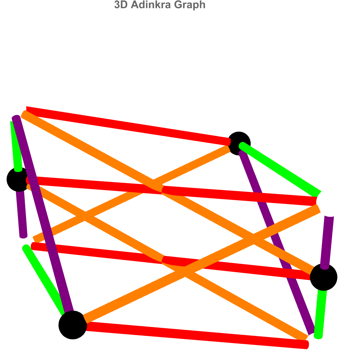
If AdrinkaGraph3D's translation of supersymmetry's algebraic data were a layered sculpture it would be radially, this anthropomorphically radialized, super healthy and physically fit just to carry, mathematical meaning--so you can literally see how each boson and fermion field intertwines through the structure of the chiral multiplet.

AdinkraVertexCoordinates[vertices_, vertexweights_] := Module[
  {coords, ids, coordsList}, 
  coords = Table[{i, j}, {i, -2, 2}, {j, -2, 2}];
  ids = Flatten[Position[vertexweights, #]] & /@ {-4, -3, -2, -1, 1, 
     2, 3, 4};
  coordsList = vertices[[#]] -> coords[[#]] & /@ ids;
  coordsList]
AdinkraGraph[vertices_, vertexweights_, edges_, edgeweights_, 
  colors_] := 
 Graph[Style[vertices[[#]], 
     If[Sign[vertexweights[[#]]] > 0, White, Black]] & /@ 
   Range[Length[vertices]], 
  Style[edges[[#]], colors[edges[[#]][[1]]], Thick] & /@ 
   Range[Length[edges]], VertexWeight -> vertexweights, 
  EdgeWeight -> edgeweights, 
  VertexCoordinates -> 
   AdinkraVertexCoordinates[vertices, vertexweights], 
  DirectedEdges -> False, ImageSize -> Medium]
vertices = {A, B, F, 
   G, \[CapitalPsi]1, \[CapitalPsi]2, \[CapitalPsi]3, \
\[CapitalPsi]4};
vertexweights = {1, 2, 3, 4, -2, -1, -3, -4};
edges = {A -> \[CapitalPsi]2, 
   B -> \[CapitalPsi]4, \[CapitalPsi]3 -> F, \[CapitalPsi]1 -> G, 
   A -> \[CapitalPsi]4, 
   B -> \[CapitalPsi]2, \[CapitalPsi]1 -> F, \[CapitalPsi]3 -> G, 
   A -> \[CapitalPsi]1, 
   B -> \[CapitalPsi]3, \[CapitalPsi]4 -> F, \[CapitalPsi]2 -> G, 
   A -> \[CapitalPsi]3, 
   B -> \[CapitalPsi]1, \[CapitalPsi]2 -> F, \[CapitalPsi]4 -> G};
edgeweights = {2, -1, 4, 3, 4, -3, -2, -1, 1, 2, -3, 2, 3, 4, 1, -2};
colors = <|1 -> Green, 2 -> Purple, 3 -> Orange, 4 -> Red|>;
HorizontalSpacing[n_] := Range[n] - (n + 1)/2;
GraphPlot3D[
 AdinkraGraph[vertices, vertexweights, edges, edgeweights, colors]]

Swapping pairs of original pairings that's the kind of thing it's like word within the word. Edges become colored, dashed or solid tubes whose hue and pattern, directly encode the magnitude and sign of the corresponding L-matrix entry. In this 3-dimensional rendition, fields are clustered by the absolute "level" of their vertex weights, arranging each group on a horizontal ring at a height equal to that level (positive weights, above, negatives below), and then, styles each node white or black by its sign.

AdinkraGraph[vertices_, edges_] := 
 Module[{n = Length[vertices], coordsList}, 
  coordsList = vertices[[#]] -> CirclePoints[n][[#]] & /@ Range[n];
  Graph3D[vertices, edges, 
   VertexStyle -> 
    Table[vertices[[i]] -> Directive[EdgeForm[Black], White], {i, n}],
    VertexCoordinates -> coordsList, ImageSize -> Medium]]
vertices = {A, B, F, 
   G, \[CapitalPsi]1, \[CapitalPsi]2, \[CapitalPsi]3, \
\[CapitalPsi]4};
edges = {A -> \[CapitalPsi]2, 
   B -> \[CapitalPsi]4, \[CapitalPsi]3 -> F, \[CapitalPsi]1 -> G, 
   A -> \[CapitalPsi]4, 
   B -> \[CapitalPsi]2, \[CapitalPsi]1 -> F, \[CapitalPsi]3 -> G, 
   A -> \[CapitalPsi]1, 
   B -> \[CapitalPsi]3, \[CapitalPsi]4 -> F, \[CapitalPsi]2 -> G, 
   A -> \[CapitalPsi]3, 
   B -> \[CapitalPsi]1, \[CapitalPsi]2 -> F, \[CapitalPsi]4 -> G};
GraphPlot3D[AdinkraGraph[vertices, edges]]

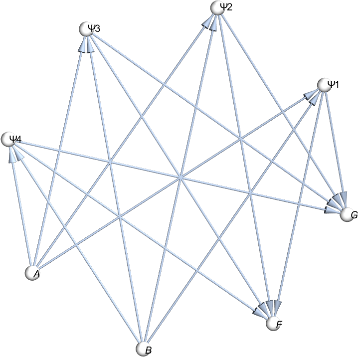
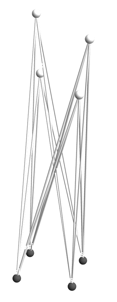
I love your visually accurate Adinkra, it's like the number of re-writing operations just isn't enough so you've got these re-writing rules. Rather than just graphing the Adinkra graph, we've collapsed the full Adinkra styling down to its bare topology--placing every node equally around a circle in the plane and rendering it in 3 dimensions as a simple white-sphere graph with black outlines. This "skeletal" AdinkraGraph strips away weights, colors, and dashed-line semantics so you can focus purely on which boson connects to which fermion, and view that connectivity from any angle. It's a minimalist textile, the adrinka, "before you even layer on its" underlying network structure before you layer on the rich supersymmetric data.

LMatricesToAdinkraGraph[L1_, X1_, Y1_, Z1_, bosons_ : {A, B, F, G}, 
  fermions_ : {Subscript[\[CapitalPsi], 1], 
    Subscript[\[CapitalPsi], 2], Subscript[\[CapitalPsi], 3], 
    Subscript[\[CapitalPsi], 4]}, n_ : 2] := 
 Module[{states, vertices, edges}, 
  states = 
   MatrixToAdinkraStates[L1, X1, Y1, bosons, fermions, n][[n + 1]];
  vertices = DeleteDuplicates@Flatten@states;
  edges = Rule @@@ states;
  AdinkraGraph[vertices, edges]]
L1 = {{1, x}, {2, w}, {3, y}, {4, z}};
X1 = {{1, z}, {2, w}, {3, x}, {4, y}};
Y1 = {{1, w}, {2, z}, {3, y}, {4, x}};
Z1 = {{-1, 0, 0, 0}, {0, -1, 0, 0}, {0, 0, -1, 0}, {0, 0, 0, -1}};

GraphPlot3D[LMatricesToAdinkraGraph[L1, X1, Y1, Z1], Boxed -> False, 
 EdgeStyle -> Directive[Thickness[0.005], Opacity[0.5]], 
 VertexSize -> Large, 
 VertexLabelStyle -> Directive[Black, FontSize -> 16], 
 PlotRange -> All, ViewPoint -> {0, -2, 1}]

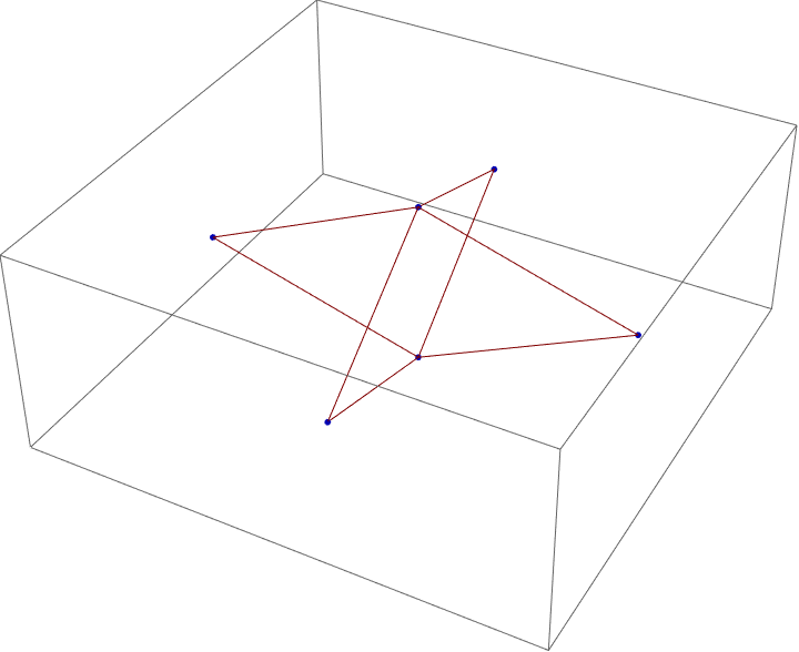
It's the supersymmetric physics from the set of L-matrices, that generate this visually accurate one and we can make smaller & larger adinkras. This function..LMatricesToAdinkraGraph elevates our Adinkra from a hand-crafted depiction into a generative, rule-driven model: by feeding in the core L-matrices and hopping operators (X1, Y1, Z1), it auto-derives the nodes and edges that define the chiral multiplet's structure, then passes them into the minimalist AdinkraGraph to demonstrate the pure connectivity in 3 dimensions. We could do the WolframModel rules or a multi-way system setup. I think that this is one of the best things that my eyes have ever seen. It's the kind of MatrixToAdinkraStates that really makes me want to, get on my hands and knees and bow down to the ground, collecting the resulting state pairs, collecting them into directed edges. The end result, is a sleek, semi-transparent 3-dimensional network, where each vertex and tube hatches directly from the algebra, so you can explore the skeleton of supersymmetry itself--no manual edge lists required.

AdinkraVertexCoordinates3D[vertices_List, vertexweights_List] := 
  Module[{groups, groupNorms, yValues, coords, n, angle, xzCoords, 
    yScale}, groupNorms = Union[Norm /@ vertexweights];
   groups = 
    GatherBy[Transpose[{vertices, Norm /@ vertexweights}], Last];
   yScale = Length[groupNorms];
   yValues = 
    Rescale[groupNorms, {Min[groupNorms], Max[groupNorms]}, {1, 
      yScale}];
   coords = {};
   Do[n = Length[groups[[i, All, 1]]];
    angle = (2 Pi)/n;
    xzCoords = 1.5*{Cos[#], Sin[#]} & /@ (angle*Range[0, n - 1]);
    coords = 
     Join[coords, 
      Thread[groups[[i, All, 1]] -> 
        Transpose[{xzCoords[[All, 1]], ConstantArray[yValues[[i]], n],
           xzCoords[[All, 2]]}]]], {i, Length[groups]}];
   Flatten[coords]];
AdinkraGraph3D[vertices_List, vertexweights_List, edges_List, 
   edgeweights_List, colors_Association] := 
  Graph3D[vertices, edges, 
   VertexStyle -> 
    Table[vertices[[i]] -> 
      Directive[EdgeForm[Black], 
       If[Sign[vertexweights[[i]]] > 0, White, Black], 
       Specularity[White, 30]], {i, Length[vertices]}], 
   EdgeStyle -> 
    Table[edges[[j]] -> {colors[Abs[edgeweights[[j]]]], 
       If[Sign[edgeweights[[j]]] < 0, Dashed, Nothing], 
       Thickness[0.008]}, {j, Length[edges]}], 
   VertexCoordinates -> 
    AdinkraVertexCoordinates3D[vertices, vertexweights], 
   ImageSize -> Large, Boxed -> False, 
   PlotLabel -> 
    Style["3D Adinkra Graph", 16, Bold, FontFamily -> "Arial"], 
   EdgeLabels -> Placed["EdgeWeight", {1/2, {0.5, 0.5}}], 
   VertexLabels -> Placed["Name", Center], VertexSize -> 0.2, 
   Lighting -> {{"Ambient", LightGray}}, ViewVertical -> {0, 1, 0}];
vertices = {A, B, F, G, Subscript[\[CapitalPsi], 1], 
   Subscript[\[CapitalPsi], 2], Subscript[\[CapitalPsi], 3], 
   Subscript[\[CapitalPsi], 4]};
vertexweights = {1, 1, 3, 3, -2, -2, -2, -2};
edges = {A -> Subscript[\[CapitalPsi], 2], 
   B -> Subscript[\[CapitalPsi], 4], Subscript[\[CapitalPsi], 3] -> F,
    Subscript[\[CapitalPsi], 1] -> G, 
   A -> Subscript[\[CapitalPsi], 4], B -> Subscript[\[CapitalPsi], 2],
    Subscript[\[CapitalPsi], 1] -> F, 
   Subscript[\[CapitalPsi], 3] -> G, A -> Subscript[\[CapitalPsi], 1],
    B -> Subscript[\[CapitalPsi], 3], 
   Subscript[\[CapitalPsi], 4] -> F, Subscript[\[CapitalPsi], 2] -> G,
    A -> Subscript[\[CapitalPsi], 3], 
   B -> Subscript[\[CapitalPsi], 1], Subscript[\[CapitalPsi], 2] -> F,
    Subscript[\[CapitalPsi], 4] -> G};
edgeweights = {2, -1, 4, 3, 4, -3, -2, -1, 1, 2, -3, 4, 3, 4, 1, -2};
colors = <|1 -> Green, 2 -> Purple, 3 -> Orange, 4 -> Red|>;
AdinkraGraph3D[vertices, vertexweights, edges, edgeweights, colors]

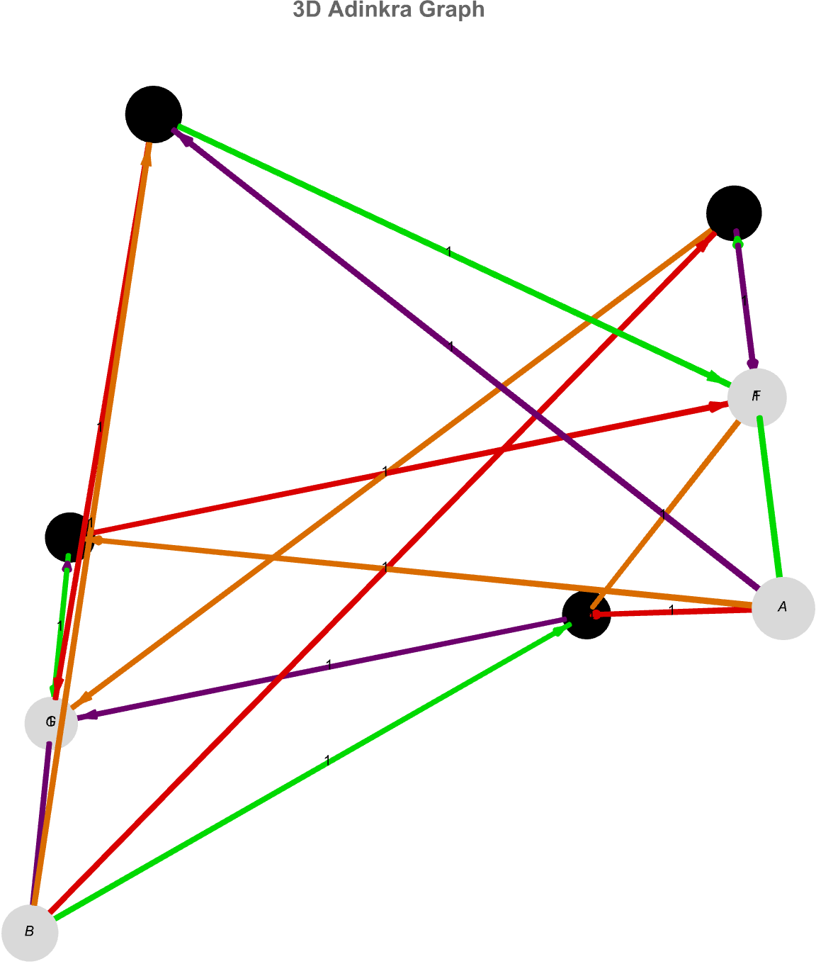
We think we know all the vertex layers but we don't, we have to map them to distinct heights but one thing we both know is that, normalizing their weight magnitudes into a 'tidy" vertical scale is what counts; each layer's nodes we evenly space in a ring around the Y-Axis which is how, positive fields gleam white, negatives solid black, both even with specular details to pop them off the backdrop, while tubes colored and dashed by edge weights arch gracefully between rings. Edge labels hover at midpoints, and vertex names sit centrally on each sphere--so you get a fully annotated, sculptural adinkra in 3 dimensions that makes the chiral multiplet's algebraic hierarchy and sign structure legible at a glance.

vertices = {A, B, F, G, Subscript[\[CapitalPsi], 1], 
   Subscript[\[CapitalPsi], 2], Subscript[\[CapitalPsi], 3], 
   Subscript[\[CapitalPsi], 4]};
vertexweights = {1, 1, 3, 3, -2, -2, -2, -2};
edges = {A -> Subscript[\[CapitalPsi], 2], 
   B -> Subscript[\[CapitalPsi], 4], Subscript[\[CapitalPsi], 3] -> F,
    Subscript[\[CapitalPsi], 1] -> G, 
   A -> Subscript[\[CapitalPsi], 4], B -> Subscript[\[CapitalPsi], 2],
    Subscript[\[CapitalPsi], 1] -> F, 
   Subscript[\[CapitalPsi], 3] -> G, A -> Subscript[\[CapitalPsi], 1],
    B -> Subscript[\[CapitalPsi], 3], 
   Subscript[\[CapitalPsi], 4] -> F, Subscript[\[CapitalPsi], 2] -> G,
    A -> Subscript[\[CapitalPsi], 3], 
   B -> Subscript[\[CapitalPsi], 1], Subscript[\[CapitalPsi], 2] -> F,
    Subscript[\[CapitalPsi], 4] -> G};
edgeweights = {2, -1, 4, 3, 4, -3, -2, -1, 1, 2, -3, 4, 3, 4, 1, -2};
colors = <|1 -> Green, 2 -> Purple, 3 -> Orange, 4 -> Red|>;
AdinkraVertexCoordinates[vertices_, vertexweights_] := 
  Module[{groups, coordsList = {}, z, m, angles, r, layerCoords, 
    currentGroup}, 
   groups = 
    GatherBy[Transpose[{vertices, Norm /@ vertexweights}], Last];
   groups = SortBy[groups, #[[1, 2]] &];
   Do[{z, currentGroup} = {groups[[i, 1, 2]], groups[[i, All, 1]]};
    m = Length[currentGroup];
    angles = Range[0, 2 Pi - 2 Pi/m, 2 Pi/m];
    r = z*0.5; 
    layerCoords = 
     Table[{r*Cos[theta], r*Sin[theta], z}, {theta, angles}];
    coordsList = 
     Join[coordsList, Thread[currentGroup -> layerCoords]], {i, 
     Length[groups]}];
   coordsList];
AdinkraGraph3D[vertices_, vertexweights_, edges_, edgeweights_, 
   colors_] := 
  Module[{vertexStyles, edgeStyles, vertexCoords, vertexShapes}, 
   vertexStyles = 
    Table[vertices[[i]] -> 
      If[Sign[vertexweights[[i]]] > 0, White, Black], {i, 
      Length[vertices]}];
   edgeStyles = 
    Table[edges[[i]] -> {colors[Abs[edgeweights[[i]]]], 
       If[Sign[edgeweights[[i]]] < 0, Dashed, Nothing], Thick}, {i, 
      Length[edges]}];
   vertexCoords = AdinkraVertexCoordinates[vertices, vertexweights];
   vertexShapes = 
    Table[If[MemberQ[{A, B, F, G}, vertices[[i]]], Sphere, Cube], {i, 
      Length[vertices]}];
   Graph3D[vertices, edges, VertexStyle -> vertexStyles, 
    EdgeStyle -> edgeStyles, VertexCoordinates -> vertexCoords, 
    VertexShapeFunction -> 
     Table[vertexShapes[[i]][#1, 0.1] &, {i, Length[vertices]}], 
    VertexLabels -> "Name", ImageSize -> Large, Boxed -> False, 
    PlotLabel -> Style["3D Adinkra Graph", 16, Bold], 
    ViewPoint -> {0, -2, 2}, Lighting -> "Neutral", 
    Background -> LightGray]];
AdinkraGraph3D[vertices, vertexweights, edges, edgeweights, colors]

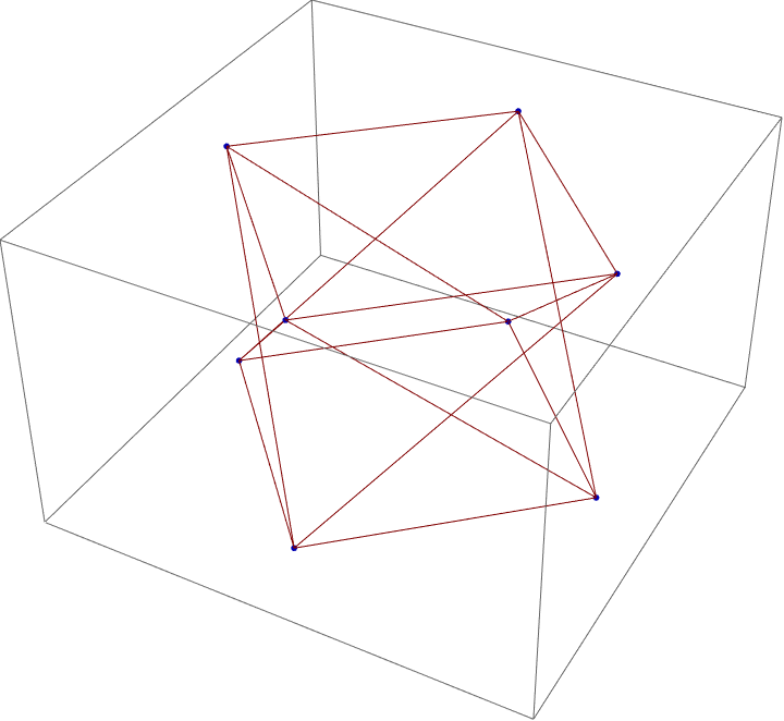
The vertices, are the eight fields four bosons, and four fermions. The vertex weights, tag each field with a level and a sign (positive for bosons & negative for fermions). The edges list each connection, from a boson to a fermion. The edge weights encode which supersymmetry generator (1-4) acts there, and the sign indicates whether the edge is solid or dashed. Also we have the color scheme that maps generator numbers to colors (Green, Purple, Orange, Red). But it's really the hard-coded coordinates that you have coords to place each node at a fixed 3-dimensional point, arranged roughly in a cube "shape" so bosons sit near the top and fermions near the bottom. In practice, this draws the supersymmetry adinkra as a labeled 3-dimensional sculpture--isn't that great? The white and black spheres connected by colored solid or dashed tubes--and then spins it around so you can see the full structure from every angle.

ClearAll[vertices, vertexWeights, edges, edgeWeights, colorScheme, 
  coords, vStyle, eStyle, graph3D];
vertices = {A, B, F, G, Subscript[\[CapitalPsi], 1], 
   Subscript[\[CapitalPsi], 2], Subscript[\[CapitalPsi], 3], 
   Subscript[\[CapitalPsi], 4]};
vertexWeights = {1, 1, 3, 3, -2, -2, -2, -2};
edges = {A -> Subscript[\[CapitalPsi], 2], 
   B -> Subscript[\[CapitalPsi], 4], Subscript[\[CapitalPsi], 3] -> F,
    Subscript[\[CapitalPsi], 1] -> G, 
   A -> Subscript[\[CapitalPsi], 4], B -> Subscript[\[CapitalPsi], 2],
    Subscript[\[CapitalPsi], 1] -> F, 
   Subscript[\[CapitalPsi], 3] -> G, A -> Subscript[\[CapitalPsi], 1],
    B -> Subscript[\[CapitalPsi], 3], 
   Subscript[\[CapitalPsi], 4] -> F, Subscript[\[CapitalPsi], 2] -> G,
    A -> Subscript[\[CapitalPsi], 3], 
   B -> Subscript[\[CapitalPsi], 1], Subscript[\[CapitalPsi], 2] -> F,
    Subscript[\[CapitalPsi], 4] -> G};
edgeWeights = {2, -1, 4, 3, 4, -3, -2, -1, 1, 2, -3, 4, 3, 4, 1, -2};
colorScheme = <|1 -> Green, 2 -> Purple, 3 -> Orange, 4 -> Red|>;
coords = <|A -> {1, 0, 2}, B -> {-1, 0, 2}, 
   Subscript[\[CapitalPsi], 1] -> {0, 2, 1}, 
   Subscript[\[CapitalPsi], 2] -> {0, -2, 1}, 
   Subscript[\[CapitalPsi], 3] -> {0, 2, -1}, 
   Subscript[\[CapitalPsi], 4] -> {0, -2, -1}, F -> {1, 0, -2}, 
   G -> {-1, 0, -2}|>;
vStyle = 
  Thread[vertices -> (If[# > 0, White, Black] & /@ vertexWeights)];
eStyle = 
  Thread[edges -> 
    MapThread[{colorScheme[Abs[#1]], If[#1 < 0, Dashed, Thick], 
       Thickness[0.009]} &, {edgeWeights}]];
graph3D = 
  Graph3D[vertices, edges, VertexCoordinates -> coords, 
   VertexStyle -> vStyle, EdgeStyle -> eStyle, VertexSize -> 0.3, 
   VertexLabels -> Placed["Name", Tooltip], 
   EdgeLabels -> Placed["EdgeWeight", Tooltip], Boxed -> False, 
   ImageSize -> 600];
Animate[Show[graph3D, 
  ViewPoint -> {4  Cos[\[Theta]], 4  Sin[\[Theta]], 2}, 
  ViewVertical -> {0, 0, 1}], {\[Theta], 0, 2  Pi}, 
 AnimationRate -> 0.05, RefreshRate -> 30]

There is a wry observation on the fact that real progress in hard sciences and technology comes from truly understanding physics principles--whether it's charged plasmas or statistical word patterns--and then artfully engineering around their stubborn obstacles. And so we have to do this for the readers, we have to make that quantum leap it's not just some "jump", it's the fact that fusion's "Sisyphean" struggle--decades of incremental progress and I mean decades, stymied by plasma instabilities, yet driven by the sun's example and the tantalizing preward of "nearly limitless" clean plower, just shows that. It just, pivots from brute-force engineering to creative physics: when materials like the Adinkra "fail", we need to lean on electromagnetic fields. It shows how fundamental, plasmas carry charge and open entirely new (technological pathways); what is fusion's "second act"? Well, "I took a class" on solving confinement "only to create new materials challenges", which "reminds me" that every breakthrough, often spawns fresh engineering "puzzles", elegantly demystifying the "automation" problems that have already been solved by higher-level languages; AI promises incremental "boosts", but not wholesale reinvention of well-engineered tools that we get; that real progress in hard sciences start fresh; each supersymmetry operator, sign indicating solid vs dashed, that's a hard-coded lookup of each node's 3-dimensional position so the graph looks like a neat octagon-cube shape. The result is an "admirable" 3-dimensional adinkra from every angle.

vertices = {A, B, F, 
   G, \[CapitalPsi]1, \[CapitalPsi]2, \[CapitalPsi]3, \
\[CapitalPsi]4};
vertexWeights = {1, 2, 3, 4, -2, -1, -3, -4};
edges = {A -> \[CapitalPsi]2, 
   B -> \[CapitalPsi]4, \[CapitalPsi]3 -> F, \[CapitalPsi]1 -> G, 
   A -> \[CapitalPsi]4, 
   B -> \[CapitalPsi]2, \[CapitalPsi]1 -> F, \[CapitalPsi]3 -> G, 
   A -> \[CapitalPsi]1, 
   B -> \[CapitalPsi]3, \[CapitalPsi]4 -> F, \[CapitalPsi]2 -> G, 
   A -> \[CapitalPsi]3, 
   B -> \[CapitalPsi]1, \[CapitalPsi]2 -> F, \[CapitalPsi]4 -> G};
edgeWeights = {2, -1, 4, 3, 4, -3, -2, -1, 1, 2, -3, 2, 3, 4, 1, -2};
colorRules = <|1 -> Green, 2 -> Purple, 3 -> Orange, 4 -> Red|>;
Adinkra3DCoordinates[vertices_, weights_] := 
  Module[{groups, coords = {}, radius = 0.8}, 
   groups = GatherBy[Transpose[{vertices, Abs /@ weights}], Last];
   Do[Module[{group = groups[[i]], norm, count, angles}, 
     norm = group[[1, 2]];
     count = Length[group];
     angles = Table[2 \[Pi]*k/count + \[Pi]/4, {k, 0, count - 1}];
     coords = 
      Join[coords, 
       Table[group[[j, 1]] -> {radius*norm*Cos[angles[[j]]], 
          radius*norm*Sin[angles[[j]]], 
          If[Positive@group[[j, 1]] /. Thread[vertices -> weights], 
           norm, -norm]}, {j, count}]]], {i, Length[groups]}];
   Association[coords]];
coords = Adinkra3DCoordinates[vertices, vertexWeights];
vertexGraphics = 
  Table[{If[vertexWeights[[i]] > 0, White, Black], 
    Sphere[vertices[[i]] /. coords, 0.15]}, {i, Length[vertices]}];
edgeGraphics = 
  Table[{colorRules[Abs[edgeWeights[[i]]]], 
    Tube[{edges[[i, 1]] /. coords, edges[[i, 2]] /. coords}, 0.04], 
    If[edgeWeights[[i]] < 0, Opacity[0.6], Opacity[1]]}, {i, 
    Length[edges]}];
Graphics3D[{edgeGraphics, vertexGraphics}, 
 Lighting -> {{"Ambient", LightGray}, {"Directional", 
    White, {{1, 1, 1}, {0, 0, 0}}}}, Boxed -> False, ImageSize -> 800,
  ViewPoint -> {2, -2, 1.5}, PlotRange -> All, 
 RotationAction -> "Clip", SphericalRegion -> True]

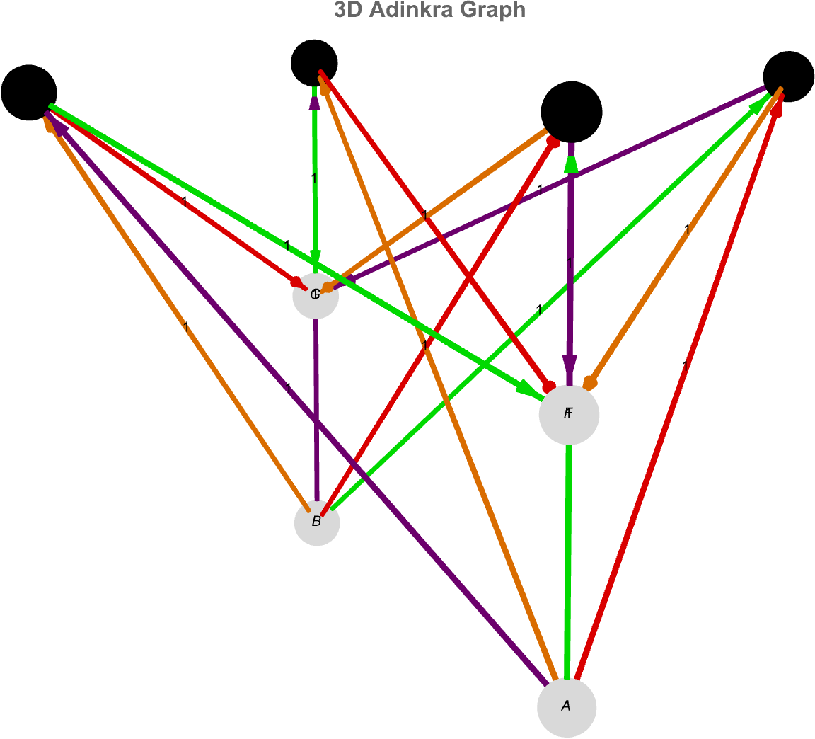
Each ring's size and height algebraically weight the sculptural structure of the adinkra, and the colored, semi-opaque tubes trace the operator connections in space. The vertices being clustered according to the absolute value of the weight, all fields at the same "deptH" form a ring, such that each ring's nodes are evenly spaced around a circle, offset by π / 4 for a pleasing tilt, the ( radius × level ) × ( cos angle, sin angle ). The Z = +level for bosons (positive weight), -level for fermions (negative weight). The supersymmetry index (1 -> Green, 2 -> Purple, 3 -> Orange, 4 -> Red), is semi-transparent "semantically" if the weight is negative (the dashed style, is replaced, by lower opacity)..and, the view point is fixed and it's fixed so you see the layered rings and the rendering, is tweaked to scale each vertex's ring radius, scale the vertex ring radius with the absolute value of its weight, and, positive-weight nodes sit above the plane while negatives, mirror them below.

vertices = {A, B, F, G, Subscript[\[CapitalPsi], 1], 
   Subscript[\[CapitalPsi], 2], Subscript[\[CapitalPsi], 3], 
   Subscript[\[CapitalPsi], 4]};
vertexweights = {1, 1, 3, 3, -2, -2, -2, -2};
edges = {A -> Subscript[\[CapitalPsi], 2], 
   B -> Subscript[\[CapitalPsi], 4], Subscript[\[CapitalPsi], 3] -> F,
    Subscript[\[CapitalPsi], 1] -> G, 
   A -> Subscript[\[CapitalPsi], 4], B -> Subscript[\[CapitalPsi], 2],
    Subscript[\[CapitalPsi], 1] -> F, 
   Subscript[\[CapitalPsi], 3] -> G, A -> Subscript[\[CapitalPsi], 1],
    B -> Subscript[\[CapitalPsi], 3], 
   Subscript[\[CapitalPsi], 4] -> F, Subscript[\[CapitalPsi], 2] -> G,
    A -> Subscript[\[CapitalPsi], 3], 
   B -> Subscript[\[CapitalPsi], 1], Subscript[\[CapitalPsi], 2] -> F,
    Subscript[\[CapitalPsi], 4] -> G};
edgeweights = {2, -1, 4, 3, 4, -3, -2, -1, 1, 2, -3, 4, 3, 4, 1, -2};
colors = <|1 -> Green, 2 -> Purple, 3 -> Orange, 4 -> Red|>;
AdinkraVertexCoordinates3D[vertices_, vertexweights_, radiusFactor_] :=
   Module[{groups, coords = {}, n, angle, r}, 
   groups = 
    GatherBy[
     Transpose[{vertices, vertexweights}], {Abs[#[[2]]], 
       Sign[#[[2]]]} &];
   Do[With[{verts = group[[All, 1]], wt = group[[1, 2]]}, 
     n = Length[verts]; r = radiusFactor*n;
     Do[angle = (k - 1)  2 \[Pi]/n;
      AppendTo[coords, 
       verts[[k]] -> {r  Cos[angle], r  Sin[angle], 
         Sign[wt]  Abs[wt]}], {k, n}]], {group, groups}];
   coords];
AdinkraGraph3D[verts_, vW_, es_, eW_, colors_, r_] := 
  Graph3D[verts, es, 
   VertexStyle -> 
    Table[verts[[i]] -> 
      If[Sign[vW[[i]]] > 0, 
       Directive[Black, Glow[White], Specularity[White, 30]], 
       Directive[GrayLevel[.3], Glow[Black], 
        Specularity[White, 30]]], {i, Length[verts]}], 
   EdgeStyle -> 
    Table[es[[i]] -> {colors[Abs[eW[[i]]]], 
       If[Sign[eW[[i]]] < 0, Dashed, Nothing], 
       Thickness[.01 + Abs[eW[[i]]]/50]}, {i, Length[es]}], 
   VertexCoordinates -> AdinkraVertexCoordinates3D[verts, vW, r], 
   VertexLabels -> Placed["Name", Center], 
   VertexLabelStyle -> Directive[Bold, 16, White], 
   EdgeLabels -> Placed["EdgeWeight", .5], 
   EdgeLabelStyle -> Directive[Bold, 12, White], ImageSize -> 200, 
   Boxed -> False, 
   PlotLabel -> Style["Interactive 3D Adinkra Graph", Bold, 12], 
   Lighting -> {{"Directional", 
      White, {{1, 1, 1}, {0, 0, 0}}}, {"Ambient", LightGray}}];
Manipulate[
 AdinkraGraph3D[vertices, vertexweights, edges, edgeweights, colors, 
  radiusFactor], {{radiusFactor, 0.3, "Layout Radius"}, 0.1, 1, .1, 
  Appearance -> "Labeled"}, ControlPlacement -> Left, 
 SynchronousUpdating -> False]

verts = {"A", "B", "F", "G", "\[Psi]1", "\[Psi]2", "\[Psi]3", 
   "\[Psi]4"};
wts = {1, 1, 3, 3, -2, -2, -2, -2};
edges = {"A" -> "\[Psi]2", "B" -> "\[Psi]4", "\[Psi]3" -> "F", 
   "\[Psi]1" -> "G", "A" -> "\[Psi]4", "B" -> "\[Psi]2", 
   "\[Psi]1" -> "F", "\[Psi]3" -> "G", "A" -> "\[Psi]1", 
   "B" -> "\[Psi]3", "\[Psi]4" -> "F", "\[Psi]2" -> "G", 
   "A" -> "\[Psi]3", "B" -> "\[Psi]1", "\[Psi]2" -> "F", 
   "\[Psi]4" -> "G"};
ewts = {2, -1, 4, 3, 4, -3, -2, -1, 1, 2, -3, 4, 3, 4, 1, -2};
colorRules = <|1 -> Green, 2 -> Purple, 3 -> Orange, 4 -> Red|>;
Manipulate[Module[{n, coords, arrows, spheres, g3}, n = Length@verts;
  coords = 
   Association@
    Table[verts[[i]] -> {radius  Cos[2  \[Pi]  (i - 1)/n], 
       radius  Sin[2  \[Pi]  (i - 1)/n], wts[[i]]}, {i, n}];
  arrows = 
   Table[With[{w = ewts[[k]]}, {Directive[colorRules[Abs[w]], 
       If[w < 0, Dashed, Thick], Opacity[edgeOpacity]], 
      Arrow[{coords[edges[[k, 1]]], coords[edges[[k, 2]]]}, 
       0.04]}], {k, Length@edges}];
  spheres = 
   Table[{If[wts[[i]] > 0, White, Black], 
     Sphere[coords[verts[[i]]], vertexSize]}, {i, n}];
  Graphics3D[{arrows, spheres}, Background -> bg, 
   Lighting -> lighting, Boxed -> boxed, SphericalRegion -> True, 
   PlotRange -> All, ImageSize -> 600]], {{radius, 2, 
   "Circle Radius"}, 0.5, 5, 0.1}, {{vertexSize, 0.2, "Vertex Size"}, 
  0.05, 1, 0.01}, {{edgeOpacity, 0.8, "Edge Opacity"}, 0.1, 1, 
  0.05}, {{bg, Transparent, "Background"}, {Black -> "Dark", 
   White -> "Light"}}, {{lighting, "Neutral", "Lighting"}, {"Neutral",
    "Accent", "Classic"}}, {{boxed, False, "Show Box"}, {True, 
   False}}, ControlPlacement -> Left]

What is the crux of every fusion approach? It's that we reach "breakeven" where output exceeds input energy--and every prediction of "ten years away" has faced skeptical odds. The problem is, the energy you spend is less than the energy you get out. That's the "second act" problem: even if you get net power, neutron "bombardment" can destroy your own machinery, demanding novel materials or liquid-metal designs. It's a "blunt" admission that tokamak research has been a seven-decade "slog": "taming" runaway plasma modes has proven the central--and fiendishly tricky--challenge, of a particle going as slowly as possible, seeing how slowly we can go out more further out in the next, orbit and so on. The kind of the king of the hearts of the magnetic-bottle fusion is that, you can't use a material object to confine a plasma. However, there's the convenient feature..you can use magnetic forces to confide the plasma. That's a bit of the outer space, type of particles wherein 'no container can withstand" 10 million °C, you conveniently corral charged particles with fields instead of walls. This contrast between fusion (building up light nuclei) and fission (splitting heavy ones) crystallizes why fusion is "so appealing"--fuel is "abundant", and the process "taps into" immense binding-energy "gains". When you go beyond iron...taking the elements apart, gives you energy.

verts = {"A", "B", "F", "G", "\[Psi]1", "\[Psi]2", "\[Psi]3", 
   "\[Psi]4"};
wts = {1, 1, 3, 3, -2, -2, -2, -2};
edges = {"A" -> "\[Psi]2", "B" -> "\[Psi]4", "\[Psi]3" -> "F", 
   "\[Psi]1" -> "G", "A" -> "\[Psi]4", "B" -> "\[Psi]2", 
   "\[Psi]1" -> "F", "\[Psi]3" -> "G", "A" -> "\[Psi]1", 
   "B" -> "\[Psi]3", "\[Psi]4" -> "F", "\[Psi]2" -> "G", 
   "A" -> "\[Psi]3", "B" -> "\[Psi]1", "\[Psi]2" -> "F", 
   "\[Psi]4" -> "G"};
ewts = {2, -1, 4, 3, 4, -3, -2, -1, 1, 2, -3, 4, 3, 4, 1, -2};
colorRules = <|1 -> Green, 2 -> Purple, 3 -> Orange, 4 -> Red|>;
Manipulate[
 Module[{coords}, 
  coords = 
   Association@
    Table[verts[[i]] -> 
      Which[i == 1, {-1, 1, bosonHeight}, i == 2, {1, 1, bosonHeight},
        i == 3, {-1, -1, bosonHeight}, i == 4, {1, -1, bosonHeight}, 
       i == 5, {-1, 1, 0}, i == 6, {1, 1, 0}, i == 7, {-1, -1, 0}, 
       i == 8, {1, -1, 0}], {i, 8}];
  Graphics3D[{Table[{Directive[colorRules[Abs[ewts[[k]]]], 
       If[ewts[[k]] < 0, Dashed, Thick], Opacity[edgeOpacity]], 
      Arrow[{coords[edges[[k, 1]]], coords[edges[[k, 2]]]}, 
       0.03]}, {k, Length@edges}], 
    Table[{If[wts[[i]] > 0, White, Black], 
      If[i <= 4, Sphere[coords[verts[[i]]], bosonSize], 
       Cuboid[coords[verts[[i]]] - {fermionSize, fermionSize, 0}/2, 
        coords[verts[[i]]] + {fermionSize, fermionSize, 0}/2]]}, {i, 
      Length@verts}]}, Lighting -> lighting, Background -> bgColor, 
   Boxed -> boxed, SphericalRegion -> True, PlotRange -> All, 
   ImageSize -> 300]], {{bosonHeight, 1, "Boson Height"}, 0, 2, 
  0.05}, {{bosonSize, .2, "Boson Size"}, 0.05, 0.5, 
  0.01}, {{fermionSize, .1, "Fermion Size"}, 0.05, 0.5, 
  0.01}, {{edgeOpacity, .7, "Edge Opacity"}, 0.1, 1, 
  0.05}, {{bgColor, Transparent, "Background"}, {Black -> "Dark", 
   White -> "Light"}}, {{lighting, "Neutral", "Lighting"}, {"Neutral",
    "Accent", "Classic"}}, {{boxed, False, "Show Box"}, {True, 
   False}}, ControlPlacement -> Left]

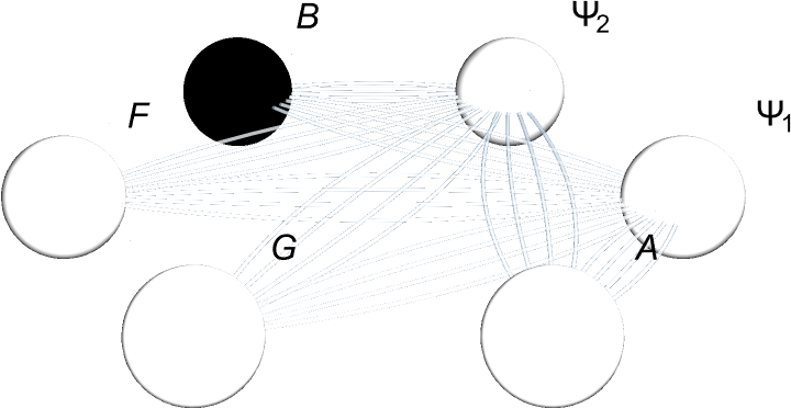
And so that is how we get this interactive, 3-dimensional picture of a small network of "boson" and "fermion" nodes connected, four bosons named A, B, F, G and four fermions labeled Ψ1-Ψ4. The node number is positive for bosons, negative for fermions (the magnitude can be used later to size or position them). edges pairs each boson with certain fermions to show who connects to whom. The sign decides dashed vs. solid, the number picks its color; a little 3-dimensional scene of four floating spheres (bosons) linked down to four cubes (fermions) by colored arrows. With just these sliders, you can raise and size the spheres, resize the cubes, the arrows fade, and you can switch the whole thing around to inspect every angle.