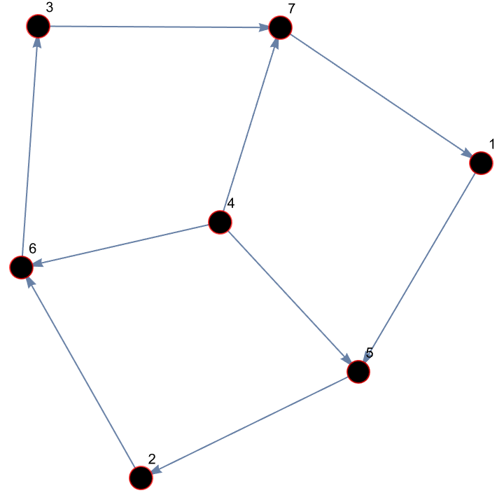
Module[{vertices, edges, graph},
vertices = {1, 2, 3, 4, 5, 6, 7};
edges = {1 -> 5, 5 -> 2, 2 -> 6, 6 -> 3, 3 -> 7, 7 -> 1, 4 -> 5,
4 -> 6, 4 -> 7};
graph = Graph[vertices, edges];
GraphPlot[graph,
VertexLabels -> All,
VertexShapeFunction -> ({EdgeForm[Red], Black, Disk[#, 0.05]} &),
VertexStyle -> Black]]
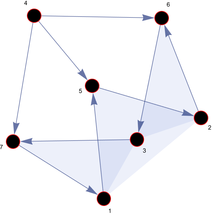
ResourceFunction["WolframModelPlot"][
{{1, 5, 2}, {2, 6, 3}, {3, 7, 1}, {4, 5}, {4, 6}, {4, 7}},
VertexLabels -> Automatic,
VertexStyle -> Directive[EdgeForm[{Red}], Black]]
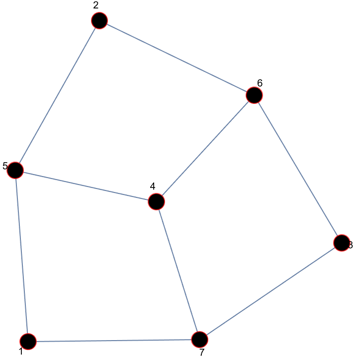
Graph[{{1, 5}, {5, 2}, {2, 6}, {6, 3}, {3, 7}, {7, 1}, {4, 5}, {4,
6}, {4, 7}},
VertexLabels -> All,
GraphLayout -> "SpringElectricalEmbedding",
VertexShapeFunction -> ({EdgeForm[Red], Black, Disk[#, 0.05]} &)]
It looks like the WolframModelPlot as we know it has vertex placements jump about between updates.
@Dugan Hammock you just need to increase the power of the LHC by a factor of ten billion...the crowds go wild when they see your silky pre-sheaves and pre-geometry lines.
GraphEmbedding is capable of simulating each vertex as one negative charge and the edges are springs.
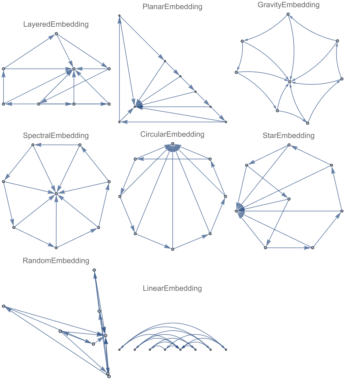
graph = Graph[{1 -> 8, 2 -> 8, 3 -> 8, 4 -> 8, 5 -> 8, 6 -> 8, 7 -> 8,
     1 -> 2, 2 -> 3, 3 -> 4, 4 -> 5, 5 -> 6, 6 -> 7, 7 -> 1}];
Graph[graph, GraphLayout -> #,
    PlotLabel -> #] & /@ {"LayeredEmbedding", "SpectralEmbedding",
   "RandomEmbedding", "PlanarEmbedding", "CircularEmbedding",
   "LinearEmbedding", "GravityEmbedding",
   "StarEmbedding"} // Multicolumn
But what if we want to use PlanarEmbedding or CircularEmbedding or even LinearEmbedding? You really allow for better visualization and understanding @Dugan Hammock when you said that vertex positions may jump around, causing some issues with visualizing the evolution.
And looking at these thin edges of the hypergraph evolution it's such a showcase being able to see the event plots stacked in ascending order. That must be why consistency is so important.
evolution =
  ResourceFunction[
    "WolframModel"][{{1, 1, 2}, {1, 3, 4}} -> {{4, 4, 5}, {5, 4,
      2}, {3, 2, 5}, {1, 6, 7}, {6, 1, 3}, {7, 2, 4}}, {{1, 1, 1}, {1,
      1, 1}, {1, 1, 1}, {1, 1, 1}}, <|"MaxEvents" -> 20|>];
What is temporal cohesion for persistent vertices? Positional cohesion comes into play and actually, there's all these mathematical structures that represent the connection between adjacent vertices. It's the conception of the 3D Graphic.
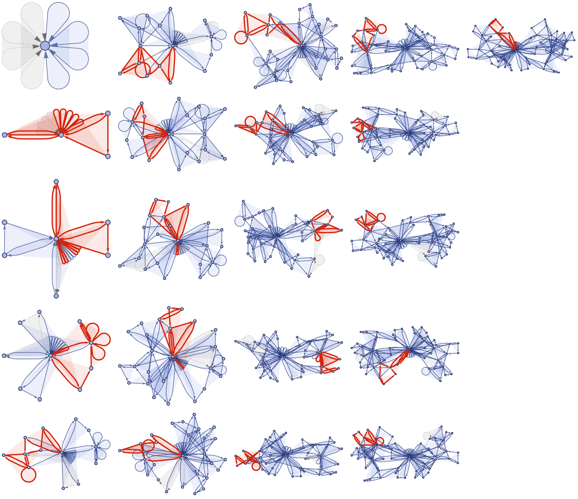
evolution["AllEventsStatesList"] // Map[ResourceFunction[ResourceObject[<|"Name" -> "WolframModelPlot", "ShortName" -> "WolframModelPlot", "UUID" -> "e8bdcbc9-6886-4c31-9f40-385a46089e07", "ResourceType" -> "Function", "Version" -> "6.0.0", "Description" -> "Generate a visual display of a hypergraph", "RepositoryLocation" -> URL["https://www.wolframcloud.com/obj/resourcesystem/api/1.0"], "SymbolName" -> "FunctionRepository`$f4c2ecb9f4ec4089b308241c70c3c877`WolframModelPlot", "FunctionLocation" -> CloudObject["https://www.wolframcloud.com/obj/a4b0555f-5c58-4299-a80e-fec09b4548ae"]|>, ResourceSystemBase -> Automatic]][#,VertexLabels->{Min[#]->Style[Min[#],Red]}]&]
So you see @Dugan Hammock this is what I strive for. Did you know that there is such a thing as temporal cohesion? For persistent vertices?
Calculate all those vertex coordinates and then we can enable visualization of the model's evolution, in 3D.
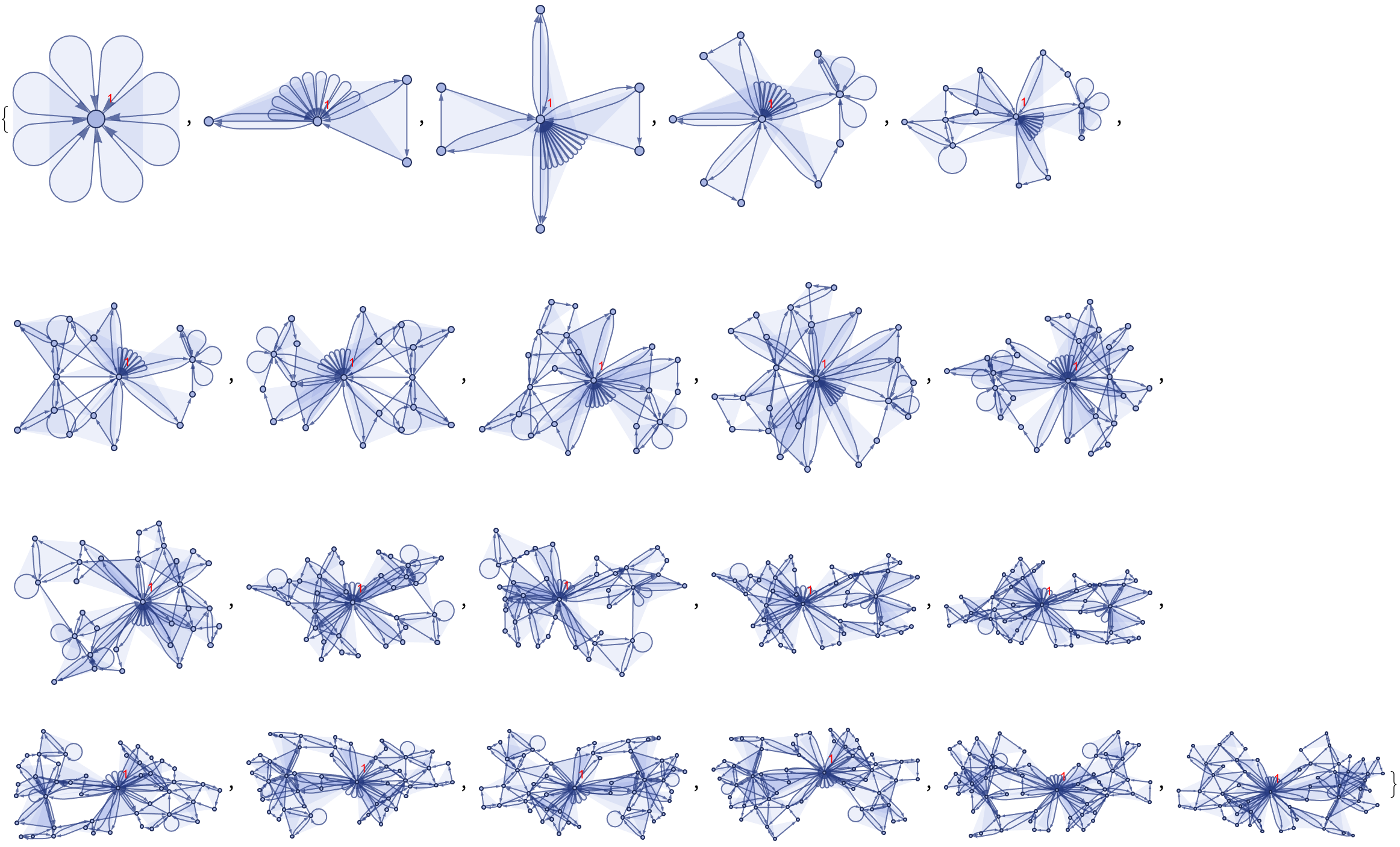
evolution["EventsStatesPlotsList"] // Multicolumn
Do you think that I should make the vertex coordinates more consistent? @Dugan Hammock .
The most interesting thing is how the z-coordinate of an event's plot, and you know it, it's identical to the z-index and the event plots can be stacked in ascending order.
Graphics[
 MapIndexed[
  Inset[#1, {20*First[#2], -20*First[#2]}, Automatic, 50] &,
  evolution["AllEventsStatesList"] // Map[ResourceFunction[
ResourceObject[<|
        "Name" -> "WolframModelPlot", "ShortName" ->
         "WolframModelPlot", "UUID" ->
         "e8bdcbc9-6886-4c31-9f40-385a46089e07", "ResourceType" ->
         "Function", "Version" -> "6.0.0", "Description" ->
         "Generate a visual display of a hypergraph",
         "RepositoryLocation" ->
         URL["https://www.wolframcloud.com/obj/resourcesystem/api/1.\
0"], "SymbolName" ->
         "FunctionRepository`$f4c2ecb9f4ec4089b308241c70c3c877`\
WolframModelPlot", "FunctionLocation" ->
         CloudObject[
          "https://www.wolframcloud.com/obj/a4b0555f-5c58-4299-a80e-\
fec09b4548ae"]|>, ResourceSystemBase -> Automatic]][#,
      VertexLabels -> {Max[#] -> Style[Max[#], Red]}] &]],
 Frame -> All,
 FrameStyle -> Gray,
 ImageSize -> Large
 ]
With regard to temporal cohesion for persistent vertices you've got this connection that ensures that the vertices' position is consistent across different states.

With[
 {
  radius = 100,
  step = 2 Pi/Length[evolution["EventsStatesPlotsList"]]
  },
 Graphics[
  MapIndexed[
   Inset[#1,
     {
      radius Cos[(First[#2] - 1) step],
      radius Sin[(First[#2] - 1) step]
      },
     Automatic,
     50] &,
   evolution["EventsStatesPlotsList"]
   ],
  Frame -> All,
  FrameStyle -> Gray,
  ImageSize -> Large]
 ]
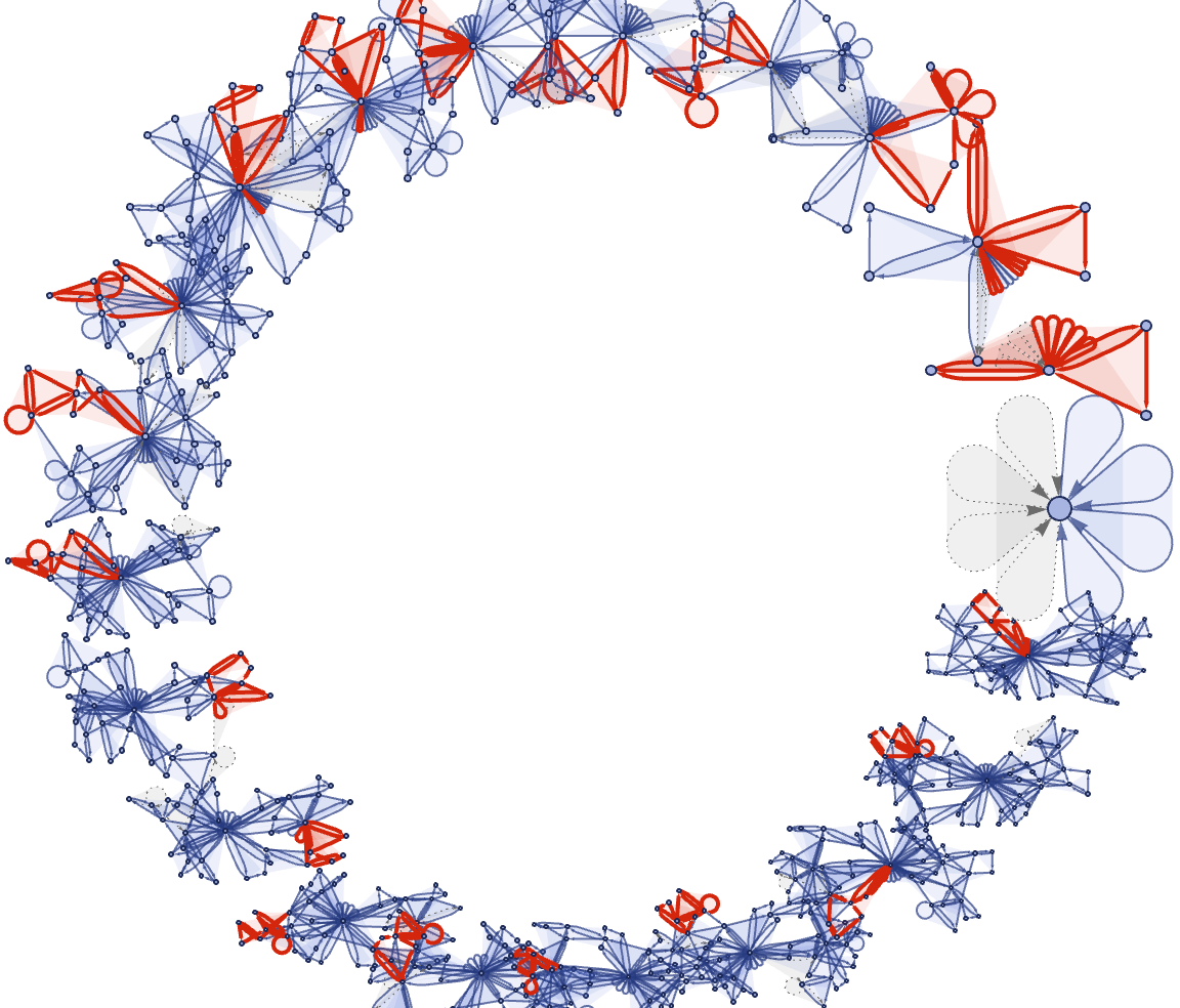
Not to mention the confinement to their respective stacked planes. And when I look at this temporal cohesion I can see all different kinds of them.
Grid[Map[
  MapAt[Style[#, Gray, Bold] &, #,
    2] &, {{Labeled[evolution["AllEventsCount"], "AllEventsCount"],
    Labeled[evolution["FinalEdgeCount"], "FinalEdgeCount"],
    Labeled[evolution["TotalGenerationsCount"],
     "TotalGenerationsCount"]}, {Labeled[
     evolution["StatesPlotsList"] // First, "First State"],
    Labeled[evolution["StatesPlotsList"] // Last, "Final State"],
    Labeled[evolution["GenerationsCount"],
     "GenerationsCount"]}, {Labeled[evolution["CausalGraph"],
     "CausalGraph"],
    Labeled[evolution["LayeredCausalGraph"], "LayeredCausalGraph"],
    Labeled[evolution["ExpressionsEventsGraph"],
     "ExpressionsEventsGraph"]}, {Labeled[
     evolution["EventsStatesPlotsList"][[1]],
     "First Generation Events"],
    Labeled[evolution["EdgeGenerationsList"] // First,
     "First Edge Generations"],
    Labeled[evolution["TerminationReason"],
     "TerminationReason"]}}, {2}], Frame -> All, FrameStyle -> Gray]
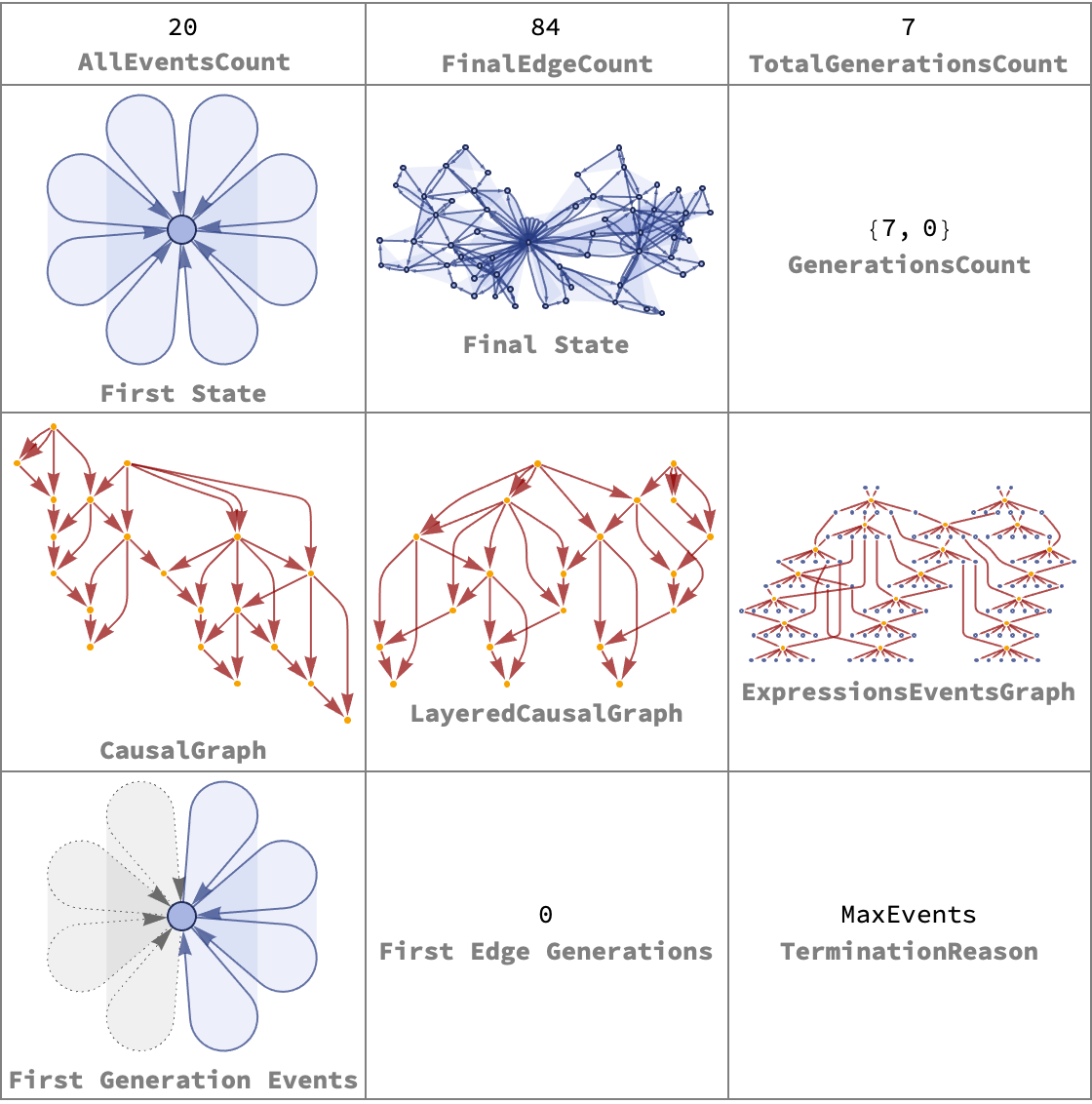
The Grid evolution persists from one state to the next CausalGraph.
WolframModelEventsPlot3D[evolution_WolframModelEvolutionObject,
  options___] :=
 Block[{eventsCount, plotsList, graphics2DLists, graphics3DLists,
   eventStateIndex}, eventsCount = evolution["AllEventsCount"];
  plotsList =
   evolution["EventsStatesPlotsList", VertexLabels -> None,
    EdgeStyle -> Green];
  graphics2DLists = plotsList // Map[First];
  graphics3DLists =
   Table[graphics2DLists[[eventStateIndex]] //
     ReplaceAll[{{x_Real, y_Real} :> {x, y, eventStateIndex - 1},
       Disk -> Sphere}], {eventStateIndex, Length[graphics2DLists]}];
  Graphics3D[graphics3DLists, Boxed -> False, options]]
WolframModelEventsPlot3D[options___][
  evolution_WolframModelEvolutionObject] :=
 WolframModelEventsPlot3D[evolution, options]
evolution =
  ResourceFunction[
    "WolframModel"][{{{1, 2, 3}} -> {{5, 3, 6}, {5, 4, 1}, {2, 3,
       2}}, {{1, 3, 2}} -> {{3, 4, 5}, {3, 6, 1}, {2, 3, 2}}, {{2, 3,
       1}} -> {{4, 6, 5}, {4, 3, 2}, {1, 3, 2}}, {{3, 1, 2}} -> {{4,
       6, 5}, {4, 3, 2}, {1, 3, 2}}, {{2, 1, 3}} -> {{3, 5, 6}, {5, 3,
        1}, {2, 3, 2}}},
   ConstantArray[{1, 1, 1}, 25], <|"MaxEvents" -> 30|>,
   "EventOrderingFunction" -> "LeastRecentEdge"];
WolframModelEventsPlot3D[evolution, ViewPoint -> {1.3, -2.4, 2.},
  BaseStyle -> EdgeForm[{Green, Thick}]] //
 Rotate[#, Pi/3, {1, 1, 1}] &
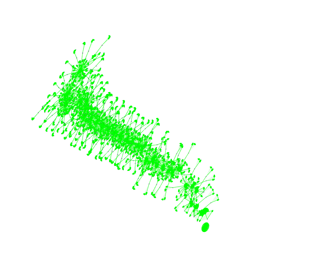
Now, when the graph vertices repel each other, and when they anchor the vertex to its previous position, and when you add the spring constant, you'll see the temporal cohesion that turns our graph inside out. I was so surprised when I saw it. There are 'world lines' which impose the tensile force, on the whole graph.


