Do you want to know what these discrete distributions with applications for coins & dice remind me of? They remind me of encyclopedias and textbooks and Cliff's Notes and so on, which were convenient never became de facto. So that's right, encyclopedias and later Encyclopedia Brittanica in Scotland, then it was Reader's Digest, then it was Cliff's Notes, and then it was all kinds of things that digest information. I agree, maybe that's the way to think about the current role of LLMs is as digesters of information. They go beyond that because you can talk to the book type thing. We build an AI tutor, specifically for Algebra I course, it's an attempt to make something that people have never made work before which is to have a purely autonomous truly scalable educational tutoring system. There's 70 years of history trying to use computers as teaching machines. It's worked great for Wolfram Alpha where you're using it as a generative content alongside what you're learning, but it's not something where the dynamics of actually teaching are delegated to the machine. It's not the way we demonstrate how Mathematica can be used to work through coin tosses and dice rolls to fishing or marble draws. It's not the toy example, it's not the 1-second cycling through quick visual checks.

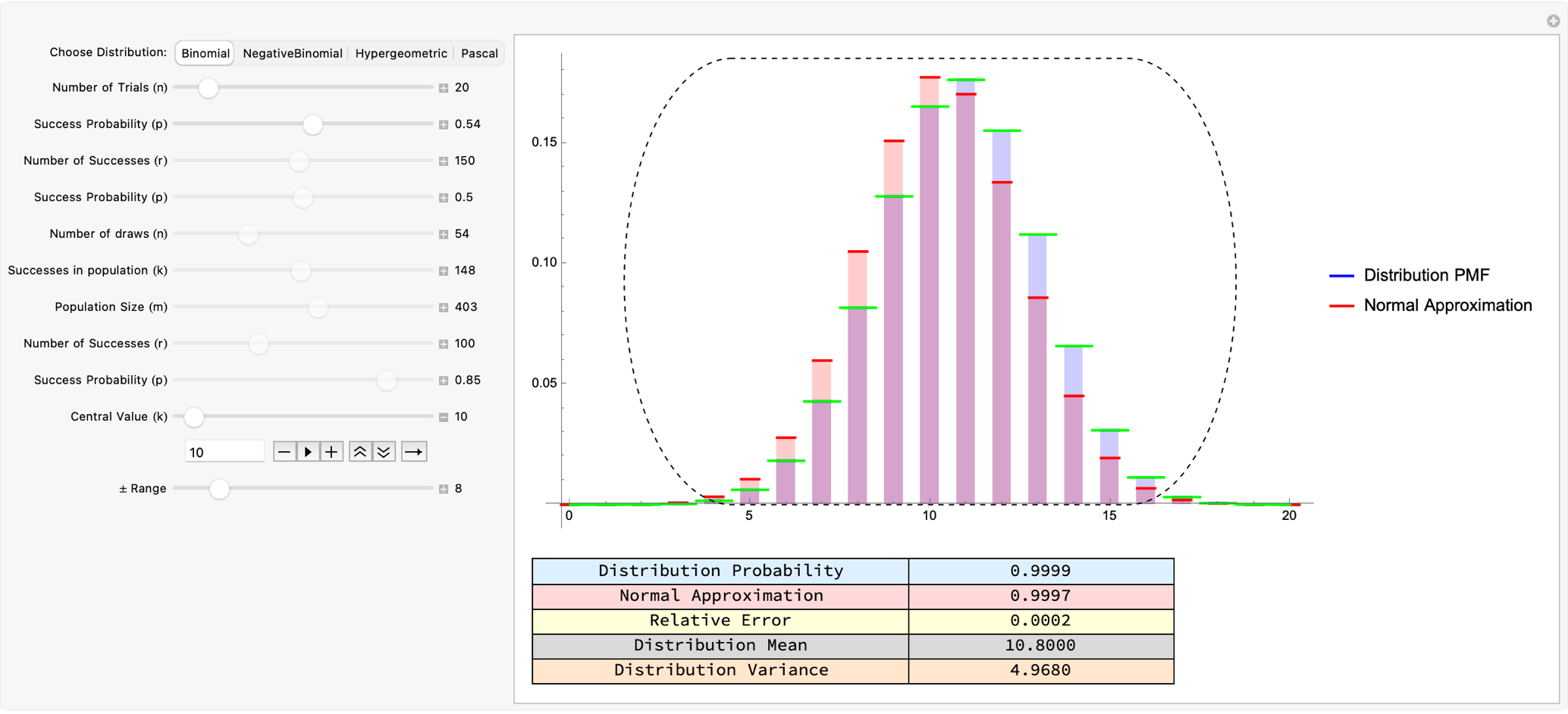
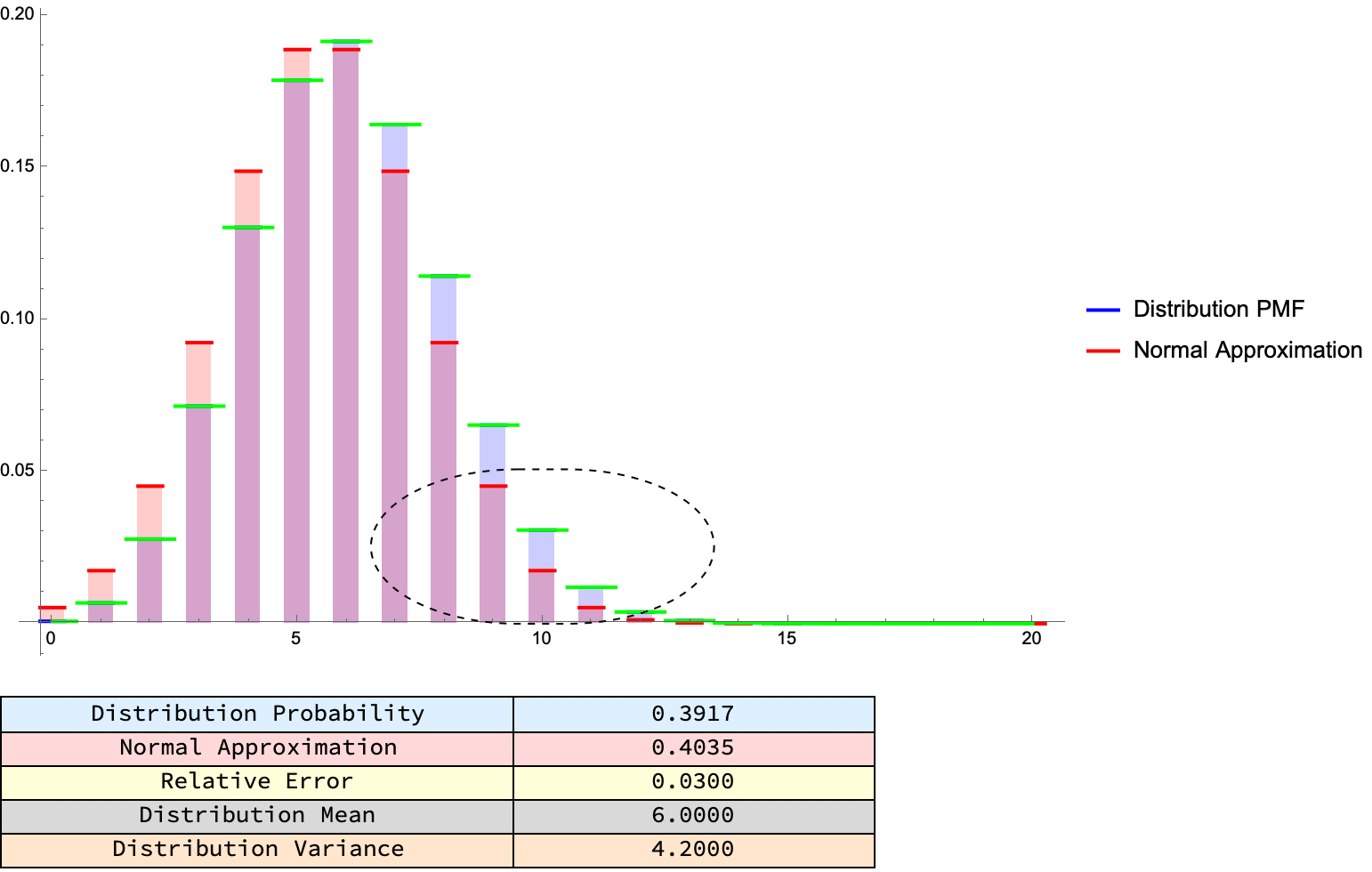
Manipulate[
 Module[{dist, mean, var, std, normalDist, xMin, xMax, probDist, 
   probNorm, relativeError, distributionPlot, pmfCurve, combinedPlot},
   If[distribution =!= oldDist, 
   dist = Switch[distribution, "Binomial", BinomialDistribution[n, p],
      "NegativeBinomial", NegativeBinomialDistribution[rNB, pNB], 
     "Hypergeometric", HypergeometricDistribution[nHyp, kHyp, mHyp], 
     "Pascal", PascalDistribution[rPasc, pPasc]];
   k = Round[Mean[dist]]; oldDist = distribution;  ];
  dist = 
   Switch[distribution, "Binomial", BinomialDistribution[n, p], 
    "NegativeBinomial", NegativeBinomialDistribution[rNB, pNB], 
    "Hypergeometric", HypergeometricDistribution[nHyp, kHyp, mHyp], 
    "Pascal", PascalDistribution[rPasc, pPasc]];
  mean = N[Mean[dist]];
  var = N[Variance[dist]];
  std = Sqrt[var];
  If[distribution === "Binomial", 
   normalDist = NormalDistribution[mean, std], normalDist = None];
  {xMin, xMax} = 
   Switch[distribution, "Binomial", {0, n}, 
    "NegativeBinomial", {0, rNB + 50}, "Hypergeometric", {0, mHyp}, 
    "Pascal", {rPasc, rPasc + 50}];
  probDist = 
   NProbability[k - bandwidth <= x <= k + bandwidth, 
    x \[Distributed] dist];
  If[distribution === "Binomial", 
   probNorm = 
    NIntegrate[
     PDF[normalDist, y], {y, k - bandwidth - 0.5, 
      k + bandwidth + 0.5}], probNorm = Missing["NotApplicable"]];
  relativeError = 
   If[distribution === "Binomial" && Abs[probDist] > 10^-12, 
    Abs[(probDist - probNorm)/probDist], Missing["NotApplicable"]];
  distributionPlot = 
   DiscretePlot[{PDF[dist, x], 
     If[distribution === "Binomial", PDF[normalDist, x + 0.5], 
      0]}, {x, xMin, xMax, 1}, PlotRange -> All, ExtentSize -> 0.5, 
    PlotStyle -> {Directive[Blue, PointSize[Medium]], 
      Directive[Red, Thick]}, Filling -> Axis, 
    PlotLegends -> 
     If[distribution === "Binomial", {"Distribution PMF", 
       "Normal Approximation"}, {"Distribution PMF"}], 
    ImageSize -> 600, 
    Epilog -> {EdgeForm[{Black, Dashed}], FaceForm[None], 
      Rectangle[{k - bandwidth - 0.5, 0}, {k + bandwidth + 0.5, 
        PDF[dist, k] + 0.02}, RoundingRadius -> 3]}];
  pmfCurve = 
   Plot[PDF[dist, Round[x]], {x, xMin, xMax}, 
    PlotStyle -> {Directive[Green, Thick]}, PlotRange -> All, 
    Axes -> False, ImageSize -> 600];
  combinedPlot = Show[distributionPlot, pmfCurve, ImageSize -> 600];
  Column[{combinedPlot, 
    Grid[Join[{{"Distribution Probability", 
        If[probDist === Missing["NotApplicable"], "-", 
         NumberForm[probDist, {\[Infinity], 4}]]}}, 
      If[distribution === 
        "Binomial", {{"Normal Approximation", 
         NumberForm[probNorm, {\[Infinity], 4}]}, {"Relative Error", 
         NumberForm[
          relativeError, {\[Infinity], 
           4}]}}, {}], {{"Distribution Mean", 
        NumberForm[mean, {\[Infinity], 4}]}, {"Distribution Variance",
         NumberForm[var, {\[Infinity], 4}]}}], Frame -> All, 
     Background -> {None, {LightBlue, LightRed, LightYellow, 
        LightGray, LightOrange}}, ItemSize -> {{20, 14}, Automatic}]},
    Spacings -> 1.5]], {{distribution, "Binomial", 
   "Choose Distribution:"}, {"Binomial", "NegativeBinomial", 
   "Hypergeometric", "Pascal"}}, {{oldDist, "Binomial"}, 
  ControlType -> None}, {{n, 50, "Number of Trials (n)"}, 1, 200, 1, 
  Appearance -> "Labeled", 
  Enabled -> Dynamic[distribution === "Binomial"]}, {{p, 0.5, 
   "Success Probability (p)"}, 0.01, 0.99, 0.01, 
  Appearance -> "Labeled", 
  Enabled -> Dynamic[distribution === "Binomial"]}, {{rNB, 150, 
   "Number of Successes (r)"}, 10, 300, 1, Appearance -> "Labeled", 
  Enabled -> Dynamic[distribution === "NegativeBinomial"]}, {{pNB, 
   0.5, "Success Probability (p)"}, 0.01, 0.99, 0.01, 
  Appearance -> "Labeled", 
  Enabled -> Dynamic[distribution === "NegativeBinomial"]}, {{nHyp, 
   54, "Number of draws (n)"}, 1, 200, 1, Appearance -> "Labeled", 
  Enabled -> Dynamic[distribution === "Hypergeometric"]}, {{kHyp, 148,
    "Successes in population (k)"}, 1, 300, 1, 
  Appearance -> "Labeled", 
  Enabled -> Dynamic[distribution === "Hypergeometric"]}, {{mHyp, 403,
    "Population Size (m)"}, 148, 600, 1, Appearance -> "Labeled", 
  Enabled -> Dynamic[distribution === "Hypergeometric"]}, {{rPasc, 
   100, "Number of Successes (r)"}, 10, 300, 1, 
  Appearance -> "Labeled", 
  Enabled -> Dynamic[distribution === "Pascal"]}, {{pPasc, 0.85, 
   "Success Probability (p)"}, 0.01, 0.99, 0.01, 
  Appearance -> "Labeled", 
  Enabled -> Dynamic[distribution === "Pascal"]}, {{k, 25, 
   "Central Value (k)"}, 0, 300, 1, 
  Appearance -> "Labeled"}, {{bandwidth, 5, "\[PlusMinus] Range"}, 1, 
  50, 1, Appearance -> "Labeled"}, 
 TrackedSymbols :> {distribution, oldDist, n, p, rNB, pNB, nHyp, kHyp,
    mHyp, rPasc, pPasc, k, bandwidth}, SynchronousUpdating -> False, 
 ControlPlacement -> Left]

What about the Wallenius' Noncentral Hypergeometric? Well, all the distributions in Mathematica (including specialized ones like WalleniusHypergeometricDistribution) let you do Probability[a <= x <= b \[Conditioned] c <= x <= d, x \[Distributed] dist]. Now, it's kind of a funny thing because for text there's trillions of words of training data. For what humans do, and how they pick things up and so on, well there's a bunch of videos you can watch but they don't have that data. And so it's kind of funny, combine the distribution with RandomVariate to generate synthetic data and show how sample histograms match up with the theoretical PMF.

Mathematica's built-in distribution functions and the synergy of Manipulate and Table let you: interactively tune parameters and see real-time changes, generate "movies" of these discrete distributions sweeping over different values and, compare the approximations e.g., Normal versus actual Probability Mass Function of discrete probability models whether it's fundamental examples like binomial coin tosses to noncentral hypergeometric "fishing" or "marble draw" problems.

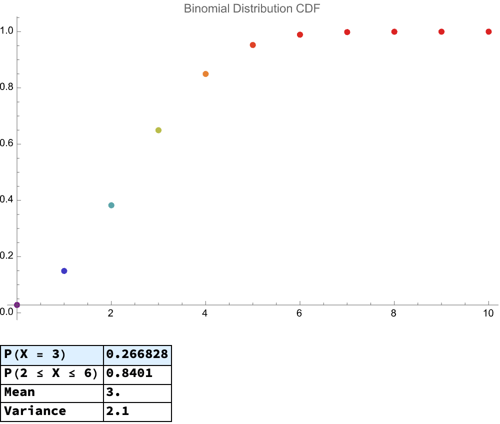
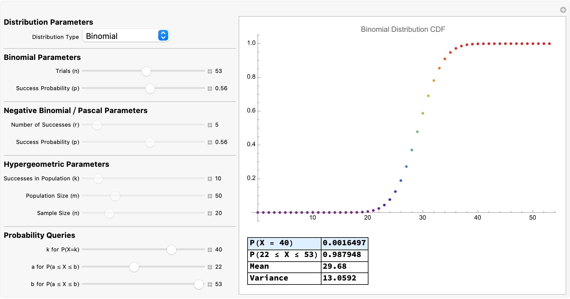
Manipulate[
 Module[{dist, cdfPlot, probTable, x}, 
  dist = Switch[distribution, "Binomial", BinomialDistribution[n, p], 
    "Negative Binomial", NegativeBinomialDistribution[r, p], "Pascal",
     PascalDistribution[r, p], "Hypergeometric", 
    HypergeometricDistribution[sampleSize, k, m]];
  cdfPlot = 
   DiscretePlot[
    CDF[dist, x], {x, 0, 
     Switch[distribution, "Binomial", n, "Negative Binomial", 
      r + 5*Ceiling[1/p], "Pascal", 3*r, "Hypergeometric", 
      Min[sampleSize, k]]}, PlotRange -> All, ImageSize -> 500, 
    Filling -> None, 
    PlotLabel -> (distribution <> " Distribution CDF"), 
    ColorFunction -> "Rainbow"];
  probTable = {{"P(X = " <> ToString[kVal] <> ")", 
     Probability[x == kVal, x \[Distributed] dist] // N}, {"P(" <> 
      ToString[aVal] <> " \[LessEqual] X \[LessEqual] " <> 
      ToString[bVal] <> ")", 
     Probability[aVal <= x <= bVal, x \[Distributed] dist] // 
      N}, {"Mean", Mean[dist] // N}, {"Variance", 
     Variance[dist] // N}};
  Column[{cdfPlot, Spacer[20], 
    Grid[probTable, Frame -> All, Alignment -> Left, Dividers -> All, 
     Background -> {None, {LightBlue, None}}, 
     ItemStyle -> {"Text", Bold}]}]], 
 Style["Distribution Parameters", Bold, 
  12], {{distribution, "Binomial", "Distribution Type"}, {"Binomial", 
   "Negative Binomial", "Pascal", "Hypergeometric"}, 
  ControlType -> PopupMenu}, Delimiter, 
 Style["Binomial Parameters", Bold, 12], {{n, 20, "Trials (n)"}, 1, 
  100, 1, Appearance -> "Labeled", 
  Enabled -> (distribution == "Binomial")}, {{p, 0.5, 
   "Success Probability (p)"}, 0.01, 0.99, 0.01, 
  Appearance -> "Labeled", 
  Enabled -> (distribution == "Binomial")}, Delimiter, 
 Style["Negative Binomial / Pascal Parameters", Bold, 
  12], {{r, 5, "Number of Successes (r)"}, 1, 50, 1, 
  Appearance -> "Labeled", 
  Enabled -> (distribution == "Negative Binomial" || 
     distribution == "Pascal")}, {{p, 0.5, "Success Probability (p)"},
   0.01, 0.99, 0.01, Appearance -> "Labeled", 
  Enabled -> (distribution == "Negative Binomial" || 
     distribution == "Pascal")}, Delimiter, 
 Style["Hypergeometric Parameters", Bold, 
  12], {{k, 10, "Successes in Population (k)"}, 1, 100, 1, 
  Appearance -> "Labeled", 
  Enabled -> (distribution == "Hypergeometric")}, {{m, 50, 
   "Population Size (m)"}, 1, 200, 1, Appearance -> "Labeled", 
  Enabled -> (distribution == "Hypergeometric")}, {{sampleSize, 20, 
   "Sample Size (n)"}, 1, 100, 1, Appearance -> "Labeled", 
  Enabled -> (distribution == "Hypergeometric")}, Delimiter, 
 Style["Probability Queries", Bold, 12], {{kVal, 10, "k for P(X=k)"}, 
  0, Dynamic[
   If[distribution == "Hypergeometric", Min[sampleSize, k], 
    If[distribution == "Binomial", n, r + 50]]], 1, 
  Appearance -> "Labeled"}, {{aVal, 5, 
   "a for P(a \[LessEqual] X \[LessEqual] b)"}, 0, 
  Dynamic[If[distribution == "Hypergeometric", Min[sampleSize, k], 
    If[distribution == "Binomial", n, r + 50]]], 1, 
  Appearance -> "Labeled"}, {{bVal, 10, 
   "b for P(a \[LessEqual] X \[LessEqual] b)"}, Dynamic[aVal], 
  Dynamic[If[distribution == "Hypergeometric", Min[sampleSize, k], 
    If[distribution == "Binomial", n, r + 50]]], 1, 
  Appearance -> "Labeled"}, ControlPlacement -> Left, 
 TrackedSymbols :> {distribution, n, p, r, k, m, sampleSize, kVal, 
   aVal, bVal}, Paneled -> True, FrameMargins -> 10]

I think @Peter Burbery, we see your textbook examples of discrete probability problems--you went from basic binomial examples to negative binomial scenarios and then the Wallenius' noncentral hypergeometric distribution for situations where each item has a different probability of being selected. I can definitely see this generalization of the (n, p) winning an award what with how you still overlap those conditional ranges and illustrate the law of large numbers and variance in samples and so on and so forth.

And I am, I'm interested in Fisher's Noncentral Hypergeometric as well as, whereas the Wallenius Noncentral Hypergeometric Distribution is most notably complex as compared to standard hypergeometric or binomial cases because each item's selection probability varies proportionally to weights..I think with the Wallenius..distribution, the conditional probability solution doesn't exactly exist however it's really Mathematica's providence of strength in handling high-precision numerical approximations, empirically distributing confirmations of theoretical results. The method of rationalizing numeric results to find Rationalize is a particularly clever approximation of extremely precise numerical outputs' validation. That's why we need AI tutors; invoking LLMs and AI tools to automatically generate, explain, or help interpret such examples is how we make complex concepts accessible to wider audiences.

Your observation regarding the lack of closed-form or exact conditional probability for Wallenius Noncentral Hypergeometric distributions suggests a real gap or open area for numerical algorithms or approximation methods to provide better analytical (or semi-analytical) solutions, leads me to believe that in your eyes @Peter Burbery, discrete distributions is a thing that you might consider turning into interactive Mathematica demonstrations (via Wolfram Demonstrations Project).

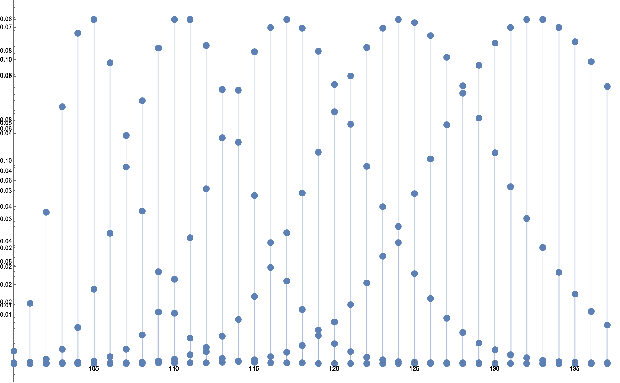
Overlay[
 Table[
  DiscretePlot[
   PDF[
    PascalDistribution[
     100,
     probab/100
     ],
    x
    ],
   {x, 100, 137},
   ImageSize -> 1000
   ],
  {probab, 75, 95, 5}
  ]
 ]
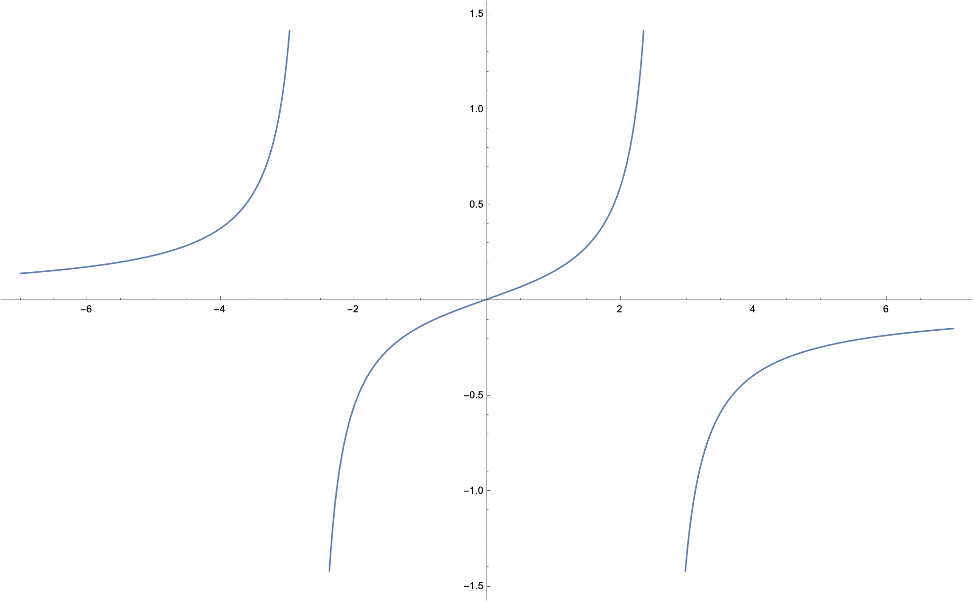
h[x_] = (RandomReal[{-1, 0}] x - RandomReal[{0, 1}])/(x^2 - 7); Plot[
 h[x], {x, -7, 7}]
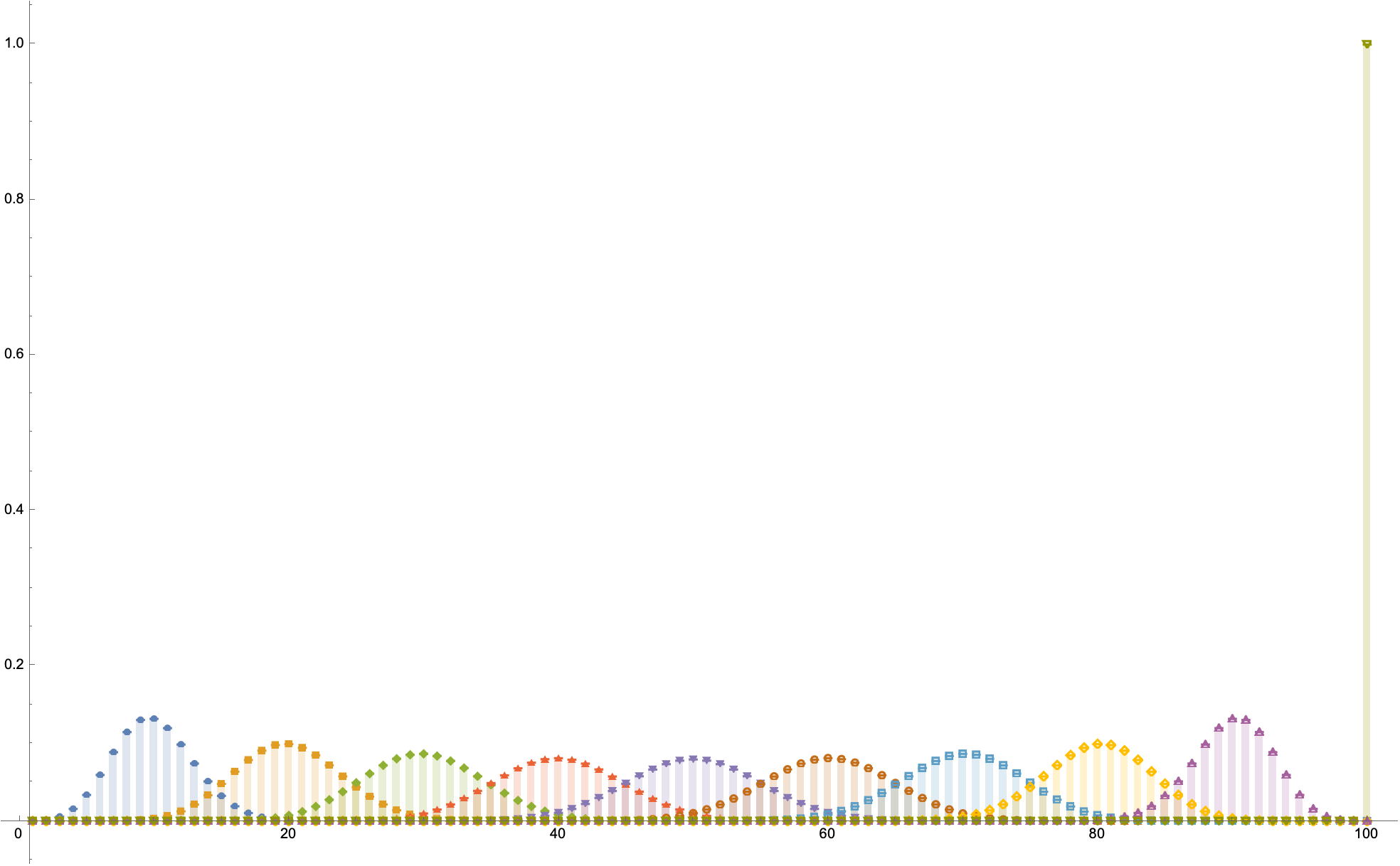
DiscretePlot[
 Table[
   PDF[
    BinomialDistribution[100, p],
    k],
   {p, Range[10]/10}
   ] // Evaluate,
 {k, 100},
 PlotRange -> All,
 PlotMarkers -> Automatic,
 ExtentSize -> 1/2
 ]

Dear Peter, we noticed your interesting plots and special type characters.

Please let us know if you need any help to make them more appealing or behave better on cloud, and please feel free to create more posts if you have ideas to share.

You might explore how generative AI (via Wolfram APIs or Mathematica) and Mathematica's interactive widgets, can discretely generate these educational visualizations: classical information summarization has a parallel with the new role of Large Language Models as modern "digesters of information" in an easily digestible format, you could build an interactive Wallenius Distribution Demo allowing users to input different weights and counts, observing how this effects probabilities. You could do a social where users select ranges and visualize conditional probabilities. I think the mathematical lucidity of your post, combined with the sheer amount of symbolic manipulation and high-precision numerical real-world applications, makes this a demonstration in and of itself.