When playing with Mathematica 10 I constructed this very simple example of an application of the NDSolve command, which I wanted to share. The objective is to model the growth of a special kind of brain tumour which affects mainly glial cells in a highly simplified way. I follow modelling ideas discussed in the excellent book "Mathematical Biology" (Vol 2) by J.D. Murray. It turns out that Gliomas, which are neoplasms of glial cells, i.e. neural calls capable of division, can be be modelled by a rather simple diffusion-growth model.
$$\frac{d c}{dt}=\nabla\left(D(x) \nabla c \right)+ \rho c$$
where c is the concentration of cancer cells and $D(x)$ is the diffusion coefficient, which depends on the coordinates; $\rho$ models the growth rate of the cells. The following boundary condition has to be observe (even though will be ignored in the model I use later on):
$${\bf n} \cdot D(x) \nabla c = 0 \qquad \text{for}\; x\; \text{on}\; \partial B.$$
In reality the diffusion coefficient will depend on the tissue type, i.e. gray matter vs white matter. I will use an image from a CT can to describe the different densities of the tissue instead.
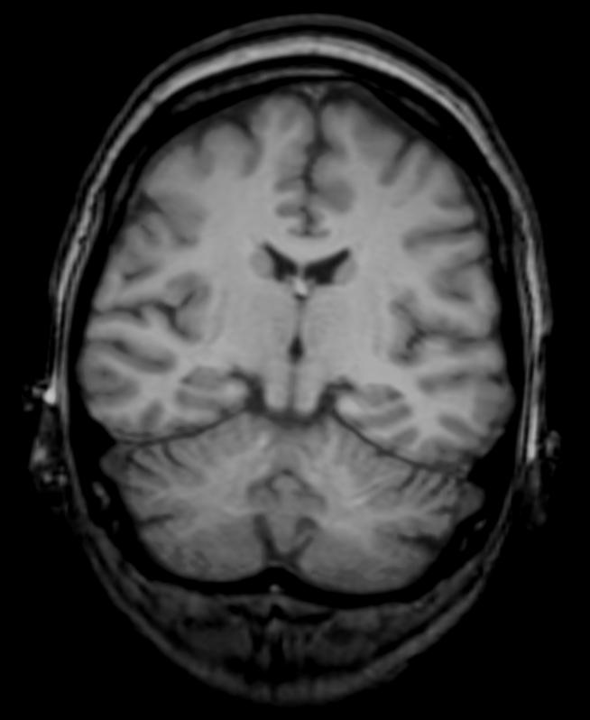
In the book by Murray great care is taken to estimate the diffusion coefficient but I just want to show the principle here. I use the attached file "brain-crop.jpg" and import it:
img2=Import["~/Desktop/brain-crop.jpg"]
Then I sharpen it and convert it to gray-scale.
img3 = Sharpen[ColorConvert[img2, "Grayscale"]]
Then I use that image to determine the diffusion coefficient, locally:
diffcoeff = ListInterpolation[ImageData[img3], InterpolationOrder -> 3]
I should now determine the boundaries using something like EdgeDetect. As the background is black and allows no diffusion at all, we can simplify this by just setting a larger (rectangular) boundary box like so:
boundaries = {-y, y - 1, -x, x - 1};

\[CapitalOmega] =
  ImplicitRegion[And @@ (# <= 0 & /@ boundaries), {x, y}];
Next we can solve the ODE on the domain:
sols = NDSolveValue[{{Div[1./500.*(diffcoeff[798.*x, 654*y])^4*Grad[u[t, x, y], {x, y}], {x, y}] - D[u[t, x, y], t] + 0.025*u[t, x, y] == NeumannValue[0., x >= 1. || x <= 0. || y <= 0. || y >= 1.]}, {u[0, x, y] == Exp[-1000. ((x - 0.6)^2 + (y - 0.6)^2)]}}, u, {x, y} \[Element] \[CapitalOmega], {t, 0, 20}, Method -> {"FiniteElement", "MeshOptions" -> {"BoundaryMeshGenerator" -> "Continuation", MaxCellMeasure -> 0.002}}]
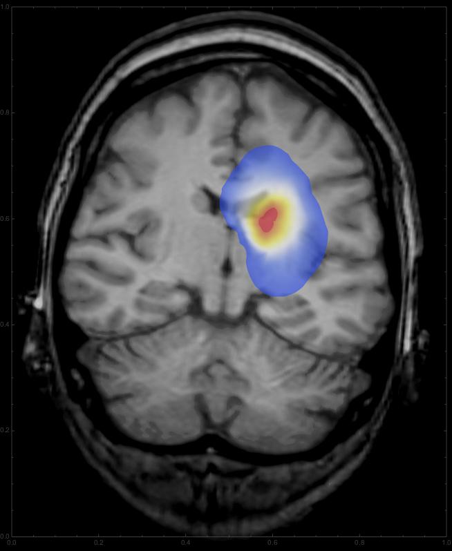
Note that we start with an initially Gaussian distributed tumour and describe its growth from there. Also I took the fourth power of the diffcoeff function, which changes the relation between grayscale and diffusion rate. You can change the coefficient to get different patterns for the growth. Interestingly, this integration gives a warning about intersecting boundaries in MMA10, which it did not say in the Prerelease version; if someone can fix that, that would be great. For any time we can now overlay the resulting distribution onto the CT image:
ImageCompose[img3, {ContourPlot[
   Max[sols[t, x, y], 0] /. t -> 2, {y, 0, 1}, {x, 0, 1},
   PlotRange -> {{0, 1}, {0, 1}, {0.01, All}}, PlotPoints -> 100,
   Contours -> 200, ContourLines -> False, AspectRatio -> 798./654.,
   ColorFunction -> "Temperature"], 0.6}]
This should give something like this:
Using
frames = Table[
   ImageCompose[
    img3, {ContourPlot[
      Max[sols[d, x, y], 0] /. d -> t, {y, 0, 1}, {x, 0, 1},
      PlotRange -> {{0, 1}, {0, 1}, {0.01, All}}, PlotPoints -> 100,
      Contours -> 200, ContourLines -> False,
      AspectRatio -> 798./654., ColorFunction -> "Temperature"],
     0.6}], {t, 0, 10, 0.5}];
we get a list of images,
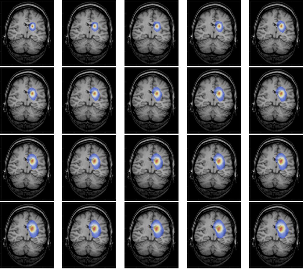
which can be animated
ListAnimate[frames, DefaultDuration -> 20]
to give
This is only a very elementary demonstration, and certainly still far away from a "real" medical application, but it demonstrates the power of NDSolve and might, in a modified form, be useful as a case study for some introductory courses.
Cheers, Marco


