Message Boards Message Boards

0
|
1297 Views
|
6 Replies
|
1 Total Likes
View groups...
Share
Share this post:

3D Plotting of Time Dilation near Black holes

Posted 5 months ago

Hi there,

I have some basic code for plotting the gravitional time dilation as one moves closer to the event horizon of a black hole of a given mass. See code:

ClearAll["Global`*"]'; tp = 1; G = 
 6.67408*10^(-11); M = (6.5*10^9)*(1.989*10^30); c = 
 2.99*10^8; rs = (2*G*
    M)/(c^2); Print[]; Print["    Black hole mass:", M, "kg", "    \
Schhwarzchild radius:", rs, "m"]; Print[]; Plot[
 tp*Sqrt[1 - (rs/r)], {r, 0, 2*10^14}, AxesLabel -> {" ", "Time (s)"},
  AxesLabel -> {Style["  (m)", Bold, 26], 
   Style["Time (s)", Bold, 16]}, LabelStyle -> Directive[Black, 16], 
 AxesOrigin -> {0, 0}, GridLines -> {{rs}, {}}, 
 GridLinesStyle -> {Directive[{Dashed, Thick}, Red], 
   Directive[Thick, Red]}, ColorFunction -> "NeonColors"]

I want to create a 3D plot for different masses of black holes ranging from the one given in the code to one a thousand times more massive, with a 3D sheet. I am not great at this, and while my basic code works fine, when I go to do a 3D plot, nothing seems to work.

Attachment

Attachments:
6 Replies

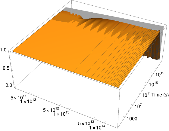
Here are just some thoughts: You can do the plot with logarithmic scaling like so:

Plot3D[tp*Sqrt[1 - ((2*G*M)/r)], {r, 0, 2*10^14}, {M, 
  1, (6.5*10^9)*(1.989*10^90)}, AxesLabel -> {" ", "Time (s)"}, 
 AxesLabel -> {Style["  (m)", Bold, 26], Style["Time (s)", Bold, 16]},
  LabelStyle -> Directive[Black, 16], AxesOrigin -> {0, 0}, 
 Filling -> {1 -> Top}, PlotRange -> All, 
 ScalingFunctions -> {"Log", "Log"}]

enter image description here

Or instead of going to very high values with the arguments you simply go straight to infinity - MMA can actually do those plots!

Plot3D[tp*Sqrt[1 - ((2*G*M)/r)], {r, 0, Infinity}, {M, 1, Infinity}, 
 AxesLabel -> {" ", "Time (s)"}, 
 AxesLabel -> {Style["  (m)", Bold, 26], Style["Time (s)", Bold, 16]},
  LabelStyle -> Directive[Black, 16], AxesOrigin -> {0, 0}, 
 Filling -> {1 -> Top}, PlotRange -> All]

enter image description here

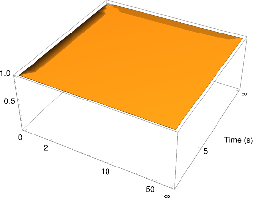
Maybe that might be on option when dealing with those very big numbers anyway.

POSTED BY: Henrik Schachner

Thanks, you got similar results to my attempt but something is wrong with the plots.

Try expressing your input in Sun masses, or something like that.

POSTED BY: Gianluca Gorni

I think I tried geometrized units but I will give it another go.

Thanks.

Very curious. Plots such as this

Plot3D[1 + (m/r), {r, 0, 10^11}, {m, 0, 10}]

give an empty box. The problem may be related to the large number 10^11. Try rescaling your problem so as to use smaller numbers.

POSTED BY: Gianluca Gorni

Indeed, hence the post. I also get an empty box.

ClearAll["Global`*"]'; tp = 1; G = 
 6.67408*10^(-11); M = (6.5*10^9)*(1.989*10^30); c = 
 2.99*10^8; Print[]; Print["    Black hole mass:", M, "kg", "    \
Schhwarzchild radius:", rs, "m"]; Print[]; Plot3D[
 tp*Sqrt[1 - ((2*G*M)/r)], {r, 0, 2*10^14}, {M, 
  1, (6.5*10^9)*(1.989*10^90)}, AxesLabel -> {" ", "Time (s)"}, 
 AxesLabel -> {Style["  (m)", Bold, 26], Style["Time (s)", Bold, 16]},
  LabelStyle -> Directive[Black, 16], AxesOrigin -> {0, 0}, 
 Filling -> {1 -> Top}, PlotRange -> 2]

The numbers have to stay the same as otherwise the plot means nothing. I even tried Log plot with no luck.

Reply to this discussion
Community posts can be styled and formatted using the Markdown syntax.
Reply Preview
Attachments
Remove
or Discard

Group Abstract Group Abstract