Message Boards Message Boards

Digital Image Correlation or Particle Image Velocimetry?

Posted 11 years ago

Hey Wolfram Community,

I would like to use Mathematica's image processing functionality to visualize the difference between these two images. Here's what's going on here: I am heating the pins, and the hot air rising from the pins is distorting the randomized background. My goal is to visualize the air plumes resulting from heating the pins.

Thus far I have tried to use ImageFeatureTrack on the two images, which gives me a list of points, but I don't know how to turn these points into a meaningful visualization on top of the original image. My ideal visualization would be lines drawn from their position in the first image to their distorted position in the second image, perhaps colored as a function of their length (i.e. areas with more distortion would have a more intense color).

I've spent about two days watching tutorials and to learn the Wolfram Language, but I'm not able to figure out which functions to use, and I keep getting errors about data types passing from one function to the next. Even an explanation of the right strategy for achieving this would be really helpful. Attached is a notebook with the two images, and my attempts so far.

Thanks, Alexander

Attachments:
4 Replies

Hey,

I just wanted to update the forum on progress. I was able to use the nuance of Photoshop to dial in the subtract features and achieve results like these.

For developing this technique, some alignment algorithms that don't deform the image could be really useful, but for me it's easier to do this manually in Photoshop than to achieve it in Mathematica.

Attachments:

Marco, thanks for such a thorough reply! It seems I was headed in the wrong direction and these images represent some great progress.

I put Mathematica down for a while and did some more research on the most algorithms to use for this problem. This article seems to demonstrate the most success, as there are several scales of phenomena visible, especially using Brox's algorithm. I have followed their instructions for capturing the images, so I think the weakness in my images is in the image-processing.
https://www.cs.ubc.ca/nest/imager/tr/2008/Atcheson_BOS_EiF/

Example Background-Oriented Schlieren Technique

The subtract function is good for making the phenomena visible, and I'm able to enhance it somewhat in Photoshop, but the underlying problem is that it is only identifying disturbance, rather than quantifying the amount of disturbance. The images are more intense where the air moves fastest, but they aren't nearly as clear as the images in this paper. Are any of the image functions capable of running more nuanced algorithms for tracking movement from one image to another?

Attachments:

By the way, this is what you get with ImageCorresponding points:

   Show[ImageResize[images[[1]], 300], 
 Graphics[{Green, Disk[#[[1]], 2]} & /@ 
   Transpose[
    ImageCorrespondingPoints[ImageResize[images[[1]], 300], 
     ImageResize[images[[2]], 300]]]], 
 Graphics[{Red, Disk[#[[2]], 2]} & /@ 
   Transpose[
    ImageCorrespondingPoints[ImageResize[images[[1]], 300], 
     ImageResize[images[[2]], 300]]]], 
 Graphics[{Thick, Line[#]} & /@ 
   Transpose[
    ImageCorrespondingPoints[ImageResize[images[[1]], 300], 
     ImageResize[images[[2]], 300]]]]]

which gives

enter image description here

so this does not really appear to be useful for you.

Cheers, Marco

POSTED BY: Marco Thiel

Hi Alexander,

I don't think that ImageFeatureTrack will work here. It is quite simple to visualise the differences between the two images:

ImageSubtract[images[[1]], images[[2]]] // ImageAdjust
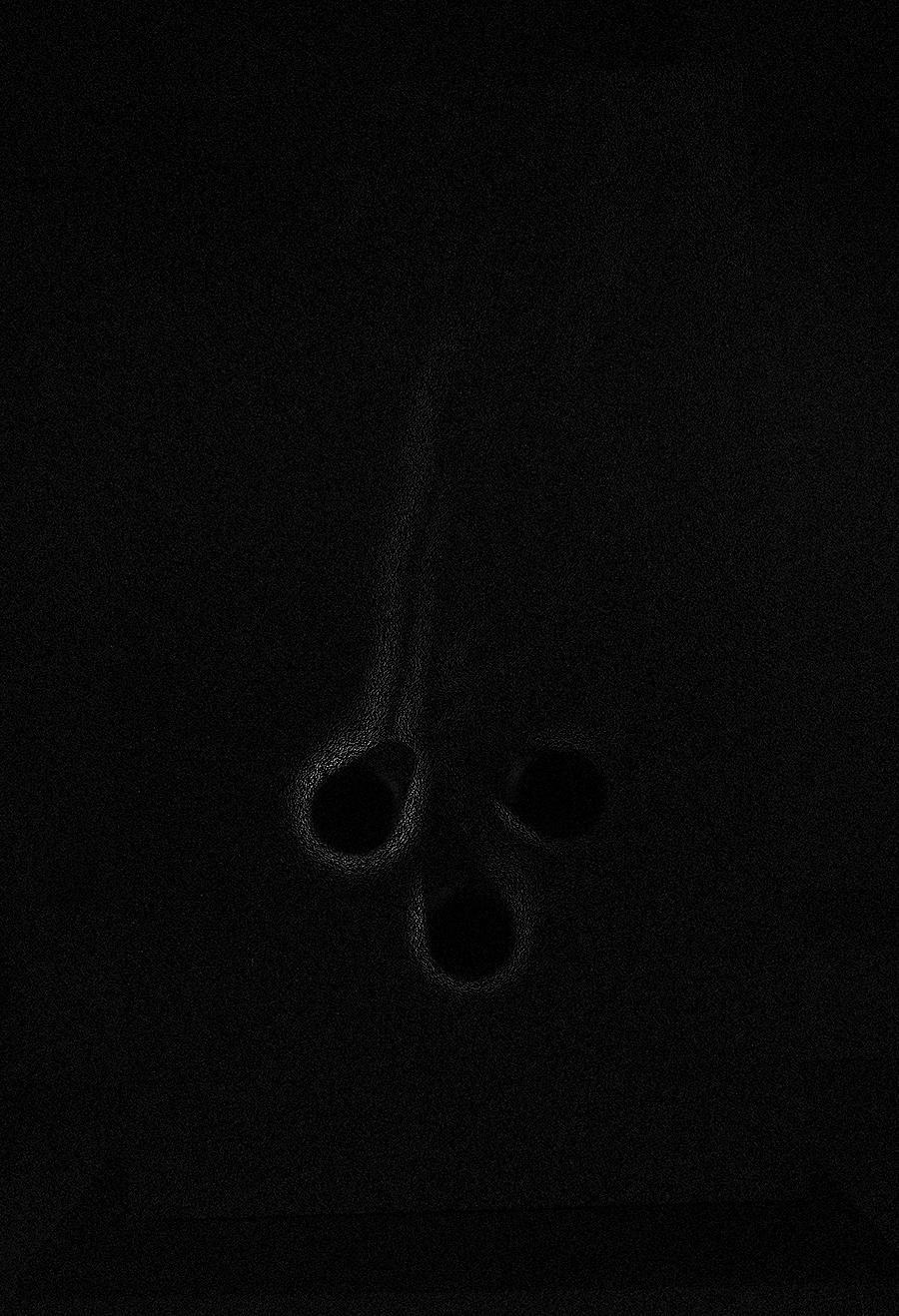
enter image description here

You can also colorise that:

Colorize[ImageAdjust[ImageSubtract[images[[1]], images[[2]]]], ColorFunction -> "ThermometerColors"]
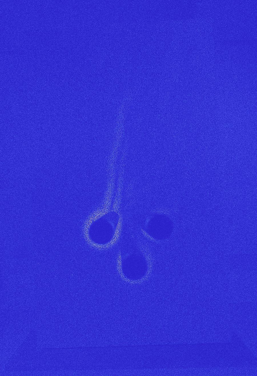
enter image description here

You can then zoom in onto one of the pins

img=ImageTrim[Colorize[ImageAdjust[ImageSubtract[images[[1]], images[[2]]]], ColorFunction -> "ThermometerColors"], {{270., 420.}, {460., 630.}}]
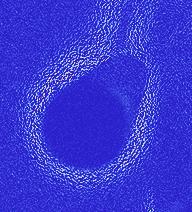
enter image description here

You can make the structures a bit clearer with

MorphologicalBinarize[img] // Colorize

I particularly like this one:

MorphologicalComponents[Binarize[img]] // Colorize
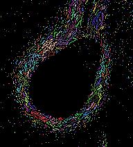
enter image description here

I know that this is not what you want, but as I said I think that ImageFeatureTrack will not work well.

If you draw the Key Points you get

Show[Graphics[{Green, Disk[#, 5]} & /@ ImageKeypoints[images[[1]]]], 
 Graphics[{Red, Disk[#, 5]} & /@ ImageKeypoints[images[[2]]]]]
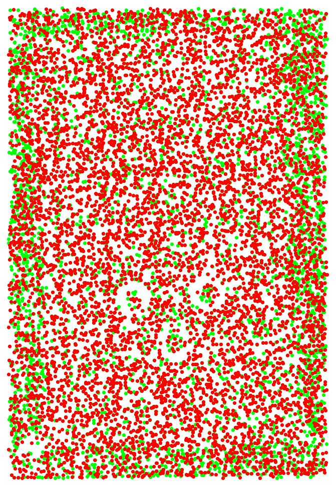
enter image description here

the thing is that even the number of key points does not match up. 7180 in one and 7186 in the other. there is no reason to assume that they "match up". In fact if you draw lines between them that looks horrible:

Graphics[Line /@ Transpose[{ImageKeypoints[images[[1]]][[1 ;; 7180]],  ImageKeypoints[images[[2]]][[1 ;; 7180]]}]]
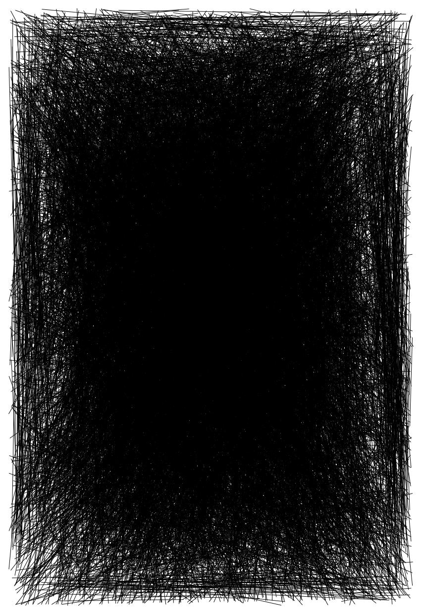
enter image description here

This command does something similar to what you want; it produces still error messages, because some points are missing, but never mind.

Show[images[[1]], Graphics[{Green, Disk[#, 5]} & /@ features[[1]]], Graphics[{Red, Disk[#, 5]} & /@ features[[2]]], Graphics[{Thick, Line[#]} & /@ 
 Transpose[{features[[1]], features[[2]]}]]]
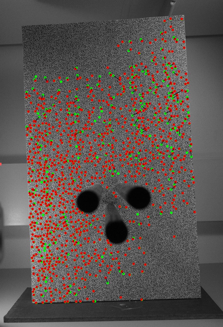
enter image description here

I can fix the missing problem if you want.

Cheers, Marco

POSTED BY: Marco Thiel
Reply to this discussion
Community posts can be styled and formatted using the Markdown syntax.
Reply Preview
Attachments
Remove
or Discard

Group Abstract Group Abstract