Message Boards Message Boards

0
|
5531 Views
|
3 Replies
|
0 Total Likes
View groups...
Share
Share this post:

How do I create a parameter-driven piece-wise function?

Posted 10 years ago

Assuming in a physic system, an object move from one point to anther point. During the movement, the acceleration changes with time t. In the first t1 seconds, a=t; In the following t2 seconds, a = 0.5t. Then I wrote the code as follows:

t1 = 1; t2 = 3;
acceleration = 
 Piecewise[{{ t, 0 <= t < t1}, {0.5 t, t1 < t <= t1 + t2}}]
velocity = Integrate[acceleration, t]
Plot[acceleration, {t, 0, t1 + t2}]
Plot[velocity, {t, 0, t1 + t2}]

And the result looks nice: enter image description here

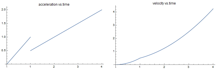
How ever, if in another application, I want to set t1 and t2 as adjustable parameter using the following code:

t1 =.; t2 =.;
acceleration = 
 Piecewise[{{ t, 0 <= t < t1}, {0.5 t, t1 < t <= t1 + t2}}]
velocity = Integrate[acceleration, t]

Then set t1=1, t2=3 and plot?

t1 = 1; t2 = 3;
Plot[acceleration, {t, 0, t1 + t2},]
Plot[velocity, {t, 0, t1 + t2}]

The result is totally different: enter image description here

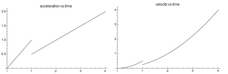
The reason why I want to set it parameter-driven is I want to get a function like v=f[t,t1,t2] which can be used in Excel calculation.

Any one could point out why in the second part of the codes doesn't the result seem reasonable?

And who can suggest a way to realize the parameter-driven system?

POSTED BY: Seasong Zhang
3 Replies

Hi,

I meant that if you run

t1 = 1; t2 = 3;acceleration = Piecewise[{{t, 0 <= t < t1}, {0.5 t, t1 < t <= t1 + t2}}];
velocity = Integrate[acceleration, t]

you get the right result and can plot it:

enter image description here

Regarding the integration see final remark in:

https://pantherfile.uwm.edu/sorbello/www/classes/mathematica_badintegral.pdf

Cheers, Marco

POSTED BY: Marco Thiel

Dear Seasong,

this is indeed not what you would expect at first. When you execute:

t1 =.; t2 =.;
acceleration = 
 Piecewise[{{t, 0 <= t < t1}, {0.5 t, t1 < t <= t1 + t2}}]
velocity = Integrate[acceleration, t]

you get

enter image description here

You see that the integral was evaluated for the three conditions individually. If you calculate

D[velocity, t]

you get the correct function of the acceleration, so that is ok. At the discontinuities there is obviously a problem with the derivative. Now if you run

t1 = 1; t2 = 3; Plot[NIntegrate[acceleration, {t, 0., tu}], {tu, 0, 4}]

you get

enter image description here

I guess that the problem is that when you execute the Integrate you have t1 and t2 not set to fixed values. If you run:

t1 = 1; t2 = 3;
acceleration = 
 Piecewise[{{t, 0 <= t < t1}, {0.5 t, t1 < t <= t1 + t2}}]
velocity = Integrate[acceleration, t]

you get

enter image description here

which gives the correct continuous plot.

Cheers, Marco

POSTED BY: Marco Thiel
Posted 10 years ago

Dear Marco,

Thanks a lot for your time and reply.

At the end of your reply, you mentioned if we set t1 and t2 to fixed values, the problem will be solved. However, what I try to do is to get the result when t1 and t2 are not fixed, which means in the output "4.25" will be a function of t1 and t2. And I want to use that function in Excel to calculate the velocity when t1 and t2 have different values.

For example, in this system, I want mathematica to give me a result like this: enter image description here

If mathematica gives such result, then I can use the formula "0.5t1^2+0.5t1 t2 + 0.25t2^2" in Excel to calculate the final velocity after two periods of acceleration without the help of mathematica any more.

Can you help? Looking forward to your reply.

POSTED BY: Seasong Zhang
Reply to this discussion
Community posts can be styled and formatted using the Markdown syntax.
Reply Preview
Attachments
Remove
or Discard

Group Abstract Group Abstract