Message Boards Message Boards

Numerically solved PDE of Ornstein–Uhlenbeck process on simplex violates conservation of probability

Posted 15 days ago

Thanks for your consideration.

I'm working to create a solution of an Ornstein-Uhlenbeck process with a force that takes mass towards the centre of a Simplex. I'm assuming absorbing boundaries.

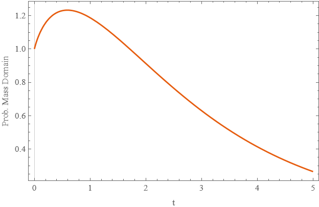
The Mathematica code below quickly provides a solution. However, the probability mass within the domain grows significantly early, but it should only ever diminish, due to mass being absorbed.

I don't think the error lies in my formulation of the forward Kolmogorov (Fokker-Plank) equation.

If it doesn't lie there, I suppose it could lie in the numerical approximation, with errors growing? I greatly appreciate any insight into this problem.

enter image description here enter image description here

ClearAll["Global`*"]

\[Eta] = 5.; (*side length*)
xopt = {\[Eta]/2, \[Eta]/(2  Sqrt[3])}; (*centroid*)
\[Kappa] = .75; (*rate of reversion to centroid,diffusion constant=1*)
Tmax = 5.; (*length of time*)


\[CapitalOmega] = 
  Polygon[Rationalize[{{0, 0}, {\[Eta], 
      0}, {\[Eta]/2, (\[Eta]   Sqrt[3])/2}}, 
    0]];  (*domain is equilateral triangle*)

bC = Rationalize[DirichletCondition[P[x1, x2, t] == 0, True], 
   0]; (*absobing boundary condition*)
iC = Rationalize[
   P[x1, x2, 0] == 
    Piecewise[{{1/((Sqrt[3]  \[Eta]^2)/4), 
       RegionMember[\[CapitalOmega], {x1, x2}]}}, 0], 
   0]; (*uniform initial condition*)

(*forward Kolmogorov equation*)
fwrdKol = 
  Rationalize[
   D[P[x1, x2, t], 
     t] == -D[\[Kappa]  (xopt[[1]] - x1)*P[x1, x2, t], {x1, 1}] - 
     D[\[Kappa]  (xopt[[2]] - x2)*P[x1, x2, t], {x2, 1}] + 
     1/2  D[P[x1, x2, t], {x1, 2}] + 1/2  D[P[x1, x2, t], {x2, 2}], 0];

(*numerical solution*)
Psol = NDSolveValue[{fwrdKol, iC, bC}, 
   P, {x1, x2} \[Element] \[CapitalOmega], {t, 0, Tmax}];


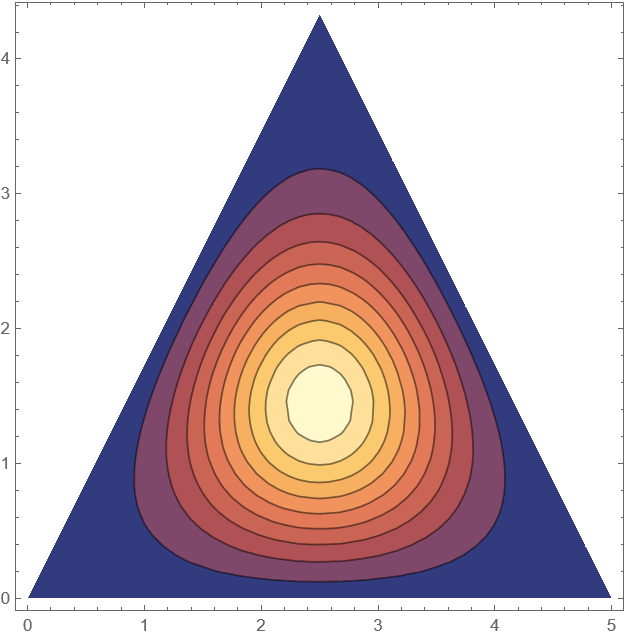
(*visualise solution at a t=Tmax/2*)
ContourPlot[Psol[x1, x2, Tmax/2], {x1, x2} \[Element] \[CapitalOmega]]

(*probability mass within domain*)
domP[t_] := 
 NIntegrate[
  Rationalize[Psol[x1, x2, t], 
   0], {x1, x2} \[Element] \[CapitalOmega], AccuracyGoal -> 4]

(*visualise*)
Plot[domP[t], {t, 0, 5}, PlotTheme -> "Scientific", PlotRange -> All, 
 FrameLabel -> {"t", "Prob. Mass Domain"}]  
POSTED BY: Cameron Turner
12 Replies

I know nothing about Kolmogorov equation. Your initial condition for P is a uniform value of 1/((Sqrt[3] \[Eta]^2)/4) over the triangle. Hence at t==0 all the spacial derivatives vanish. Now the initial time derivative of P is positive everywhere on the triangle:

fwrdKol /. t -> 0 /.
 {P[x1, x2, 0] -> 1/((Sqrt[3]   \[Eta]^2)/4),
  Derivative[_, _, 0][P][__] :> 0}

No surprise that the integral of P increases at the start.

An unrelated question: what is the purpose of all those Rationalize? Why don't you start with exact values for the parameters?

POSTED BY: Gianluca Gorni

It seems reasonable that the mesh needs to be very fine only near the boundary, where the initial datum is discontinuous. You may try the option MeshRefinementFunction.

The purpose to make the input exact instead of floating-point is good. In your case it could be done more easily by giving exact parameters at the start. Instead of floating point values, as in

\[Eta] = 5.; 
\[Kappa] = .75; 
Tmax = 5.;

I would suggest

\[Eta] = 5; 
\[Kappa] = 3/4; 
Tmax = 5;

This way there is no need for Rationalize. Even more: with your original floating-point \[Eta] = 5. the triangle definition

\[CapitalOmega] = 
  Polygon[Rationalize[{{0, 0}, {\[Eta], 
      0}, {\[Eta]/2, (\[Eta]   Sqrt[3])/2}}, 
    0]]

actually decreases the precision, because \[Eta] Sqrt[3])/2 becomes first floating-point, and then Rationalize freezes the approximation instead of the exact value.

POSTED BY: Gianluca Gorni

I would suggest to discretize the triangle so that the elements are smaller near the boundary:

\[CapitalOmega]Discretized = 
 DiscretizeRegion[\[CapitalOmega], 
  MeshRefinementFunction -> 
   Function[{vertices, area}, 
    area > 0.1 (RegionDistance[RegionBoundary[\[CapitalOmega]], 
        Mean[vertices]])]]

Instead of 0.1 you can use a smaller parameter, with longer computing time and hopefully better precision. Try using \[CapitalOmega]Discretized instead of \[CapitalOmega].

The time derivative of P is strongly negative near the boundary, enough to counteract the positive value inside:

Plot3D[Derivative[0, 0, 1][Psol][x1, x2, .01],
 Element[{x1, x2}, \[CapitalOmega]Discretized]]
POSTED BY: Gianluca Gorni

Hi Cameron, I agree with you that your formulation of the problem and your PDEs look correct. If you plot your solution over time at one of the boundary points such as P(0,0,t), it looks like Mathematica is setting the boundary conditions to be P(0,0,t)*e^(-t) with the coefficient (-1) being exact. This is quite annoying, but you can remedy it by explicitly setting the boundary condition to P(0,0,t)*e^(-10000*t).

bC = Rationalize[
   DirichletCondition[
    P[x1, x2, t] == Exp[-10000  t] 1/((Sqrt[3]   \[Eta]^2)/4), True], 
   0]; 

In the study of linear PDEs this discontinuity (setting P(x,y,0)=const. on the domain and P(x,y,t)=0 on the boundary) isn't much of an issue and it's standard to do, so it's frustrating that Mathematica makes such a big deal about it! At least with this fix applied you can see that the derivative of the total probability mass approaches -infinity near t=0, so that hints at some potential numerical difficulties.

POSTED BY: David Moore
Posted 14 days ago

Update: This is my first foray into numerically solving PDEs, I am learning as I'm troubleshooting. I have tried drastically refining the mesh, accuracy, and step size. This hasn't lessened the violation of conservation, perhaps indicating a problem in formulation. But I've been fastidious with that as well, and can't find a problem.

POSTED BY: Cameron Turner
Posted 14 days ago

Update 2: My formulation of the differential equation matches that produced automatically by Mathematica

eqn = ItoProcess[{\[DifferentialD]x1[
      t] == \[Kappa] (x1opt - 
        x1[t])  \[DifferentialD]t + \[DifferentialD]w1[
       t], \[DifferentialD]x2[
      t] == \[Kappa] (x2opt - 
        x2[t])   \[DifferentialD]t + \[DifferentialD]w2[t]}, {x1[t], 
   x2[t]}, {{x1, x2}, {x10, x20}}, 
  t, {w1 \[Distributed] WienerProcess[], 
   w2 \[Distributed] WienerProcess[]}]

eqn["KolmogorovForwardEquation"] // TraditionalForm 
POSTED BY: Cameron Turner
Posted 14 days ago

The initial condition was inconsistent and needed to exclude the boundary:

iC = Rationalize[
   P[x1, x2,0] == 
    Piecewise[{{1/
        Area[\[CapitalOmega]], (RegionMember[
           RegionBoundary[\[CapitalOmega]], {x1, x2}] == False \[And] 
         RegionMember[\[CapitalOmega], {x1, x2}])}}, 0], 0];
POSTED BY: Cameron Turner

I am totally ignorant on numerical methods for PDEs, but I wonder what accuracy you can expect with discontinuous initial data.

POSTED BY: Gianluca Gorni
Posted 13 days ago

Hi Gianluca,

  1. I'm still figuring out the accuracy of the solution, but for the 1D case the FEM and Method of Lines numerical solutions closely agree. If you make the mesh very fine (.001) it is generating reasonable results (e.g. 1> total probability >.99).

  2. The purpose of Rationalize is to make the input into the numerical solver infinite precision rather than machine precision. It's recommended in some videos on WolframU (i'm doing it pretty ritualistically at the moment).

  3. After having correctly specified the problem the integral does always decrease as expected. No matter the domain, the Kolmogorov (Fokker-Plank) equation describes a conservative system, so there should never be an increase.

enter image description here

POSTED BY: Cameron Turner
Posted 12 days ago

That's a great point regarding rationalising the parameters only, I'll be instituting that.

I'll have to think a bit more about how to square your point about spatial derivatives with the fact that mass evidently does decrease within the domain. I'll get back when I have a decisive answer, but one thing to note is that the flux of probability is in the opposite direction to the gradient of $$p$$

POSTED BY: Cameron Turner

Thanks Gianluca!

POSTED BY: Cameron Turner

Thanks David, this is really great input! I think this along with the comments above practically solves the problem!

POSTED BY: Cameron Turner
Reply to this discussion
Community posts can be styled and formatted using the Markdown syntax.
Reply Preview
Attachments
Remove
or Discard

Group Abstract Group Abstract