Foreword:
Hello Everyone,
I am Levente Fekésházy, a PhD student at the University of Hamburg and Eötvös Loránd University. My research focuses on precision quantum chromodynamic calculations, which heavily rely on symbolic algebra programs like Wolfram Mathematica. As my PhD approaches its end, I've decided to share a few tricks to handle large symbolic expressions in Mathematica.
If we're dealing with massive expressions, why not switch to FORM?
While many researchers in high energy physics prefer FORM over Mathematica, it suffers from a critical limitation: functionality. FORM implements only a handful of high-level functions (though the recent version can interface with Flint). In contrast, Mathematica offers an extensive ecosystem of high energy physics packages like LinApart, alibrary, MultivariateApart, MT, HPL, PolylogTools, HypExp, Diogenes, FeynCalc etc. Furthermore, there are powerful built-in functions which are extremely useful and save us both time and energy. Hence, it is all about convenience. Research timelines and funding rarely allow the reinvention of the wheel... or hundreds of wheels. While the physics community could theoretically port all necessary tools to FORM; and individual researchers have likely implemented many already, publication pressure discourages code sharing. Thus, for a newbie like a PhD student it is extremely hard to start their research.
What is the problem with Mathematica?
Mathematica's Achilles' heel is performance. Many functions critical to high energy physics haven't been optimized in over a decade. Meanwhile, computational demands have exploded: where "large" once meant thousands of terms, we now routinely handle several millions. Some issues for example:
Mathematica stores everything in RAM, even when file-based storage would be more practical for massive expressions.
Despite keeping data in memory, Mathematica handles substitutions far slower than FORM, which processes terms individually from disk.
Parallelization is a nightmare, the overhead both at the start and end of calculations render the well-known parallel functions like ParallelTable or Parallelize impractical in computer algebra calculations.
Expand is one, if not the most basic function of a computer algebra calculation. However it is painstakingly slow in Mathematica; there is no nicer way to put it. Even Maple's expanding function is significantly faster, let alone FORM's. I only see two possibilities why it can be so:
they sort too many times. This is confirmed by the documentation of Distribute, where it states, that Expand sorts after every step; which is the worst way to do it.
it uses an old sorting algorithm and it wasn't updated to a newer one, for example to power-sort.
Despite the limitations, Mathematica remains an invaluable tool. Its intuitive syntax and gentle learning curve make it accessible, while its comprehensive functionality makes it indispensable. The key to success lies in optimization. While each calculation is unique, certain optimization strategies are valid in general. This guide focuses on two frequently-used functions/operations, Series and Apart, to demonstrate various optimization techniques and their dramatic impact on performance. These examples will show how careful handling of the expressions can keep Mathematica working even with "larger" expressions.
Notes:
These "tricks" are well known in the community and many, like gathering and making coefficients symbolic, have their own built-in functions even in FORM. My main goal is to spare some time and flatten the learning curve of the language for newcomers. Thus, I would like to ask the advanced users to refrain themselves from comments like:
                   > ThiS Is TRiVial!!!4!!!
                   > EvERyBODy HaS a FuNCtioN FoR THis!
In each section I will - try to motivate and introduce the philosophy very shortly, - then present the functions themself, because I believe it is important, that one can see it is not magic. - lastly I will present some examples.
The code and the examples can be found on my GitHub at
https://github.com/fekeshazy/How_to_handle_big_expressions_in_Mathematica
I will not explain every line of each function, since my goal is to showcase the functionality and not to write a Mathematica lecture note. However, I tired to extensively comment the code and structure it such a way, that one can understand it after giving it some thought.
I also leave out some edge-cases, error messaging and similar things in order to not clutter up the text further. Thus, these are not finished functions, in order to release them to a general userbase one must massage them a bit.
I do not hold myself to strict standards here, thus it can happen that some parts of the codes are redundant and or can be written nicer and or be optimized.
Gathering:
Motto: If computers rebel, the first to be executed will be the programmers who write unoptimized code.
Motivation:
When we are working with big expressions, we must think about optimization; the first question is to ask ourselves: how would I do it? And I can assure you, if you were given a huge sum you would try to avoid doing the same calculation many times. However, our two example functions Apart and Series applies itself on every term... always... hence it does the same calculation over and over again in some cases. The situation is even worse, there is no built-in function in Mathematica, like Bracket in FORM, which would organize the expression in a way, that said functions only be applied on the variable dependent parts. What do I mean by this exactly? Let us take the following expression:
A/(x-1)/(x-2)+B/(x-1)/(x-2)+C/(x-4)/(x+5),
if we want to partial fraction it Apart will be applied on all of the terms individually, but then we would do Apart[1/(x-1)/(x-2),x] twice. On paper, one would immediately do the
A/(x-1)/(x-2)+B/(x-1)/(x-2)+C/(x-4)/(x+5) -> (A+B)/(x-1)/(x-2)+C/(x-4)/(x+5)
bracketing to avoid this. Of course, we have the Collect function but that has three drawbacks:
- we cannot apply a function on the variable dependent part,
- it can only separate terms by pattern,
- it brackets everything, so we are not getting a separation by unique structures.
The first means, we cannot just write
A/(x-1)/(x-2)+B/(x-1)/(x-2)+C/(x-4)/(x+5)//Collect[#, a_/;FreeQ[a,x]&, #&, Apart[#,x]& ]&
to partial fraction the expression.
The second, a_/;FreeQ[a,x]& pattern makes it immensely inefficient in the large term limit.
Furthermore, we need separation by unique parts, not just for Series or Apart, but also in order to use some rules, like the ones for integrating polylogarithms. So if we have:
na+nb x + x G[x]+ 2 na nb x + na^2x G[x]+x^2+x^2G[x]//Collect[#,x]&
and we get
na + x^2 (1 + G[x]) + x (nb + 2 na nb + G[x] + na^2 G[x])
we cannot directly apply a rule like x^pow_. G[x] -> (...) .
Thus, we ought to write our own function, which must also be at least as fast or faster than Collect.
Code:
I) Identifying the dependent terms.
- We have to expand our expression to get every dependency explicit; for that, we can use the second argument of expand.
- Convert it to a list.
Separate the dependent and independent multiplicative terms.
 ClearAll[Dependent]

          (*If the expression is free of the variable give back the expression.*)
 Dependent[expr_,var_]:={expr,1}/;FreeQ[expr,var]

          (*
                   -expanding of expression,
                   -making it a list; edge case when we only have a multiplication not a sum
                   -separate the variable dependent terms.
          *)
 Dependent[expr_,var_]:=Block[
          {
          tmp=expr
          },

         tmp=tmp//Expand[#,var]&;
         tmp=If[Head[tmp]===Plus,List@@tmp,{tmp}];
         tmp=SeparateDependency[#,var]&/@tmp

 ]


          (*
          This function separates the dependent part of an expression. This only works on single expression! Thus,
          expressions without any addition in the numerator and expressions which head is not Plus!

          The first 4 rules are for the special cases, when Select cannot be used. Like when:
                   1. the expression is only one term;
                   2. the expression is a fraction, with one term in the numerator and one in the denominator.
          *)

 ClearAll[SeparateDependency]

          (*The expression is a special case and is free of the variable.*)
 SeparateDependency[expr_,var_]:={expr,1}/;Head[expr]=!=Times&&FreeQ[expr,var]
 SeparateDependency[expr_,var_]:={expr,1}/;Length[expr]===0&&FreeQ[expr,var]
 SeparateDependency[expr_,var_]:={expr,1}/;Length[expr]===2&&Head[expr]===Power&&FreeQ[expr,var]

          (*The expression is a special case and is not free of the variable.*)
 SeparateDependency[expr_,var_]:={1,expr}/;Head[expr]=!=Times&&!FreeQ[expr,var]
 SeparateDependency[expr_,var_]:={1,expr}/;Length[expr]===0&&!FreeQ[expr,var]
 SeparateDependency[expr_,var_]:={1,expr}/;Length[expr]===2&&Head[expr]===Power&&!FreeQ[expr,var]

          (*The expression is a multiplication.*)
 SeparateDependency[expr_,var_]:=expr//{#//Select[#,FreeQ[#,var]&]&,#//Select[#,!FreeQ[#,var]&]&}&
II) Writing the front of the function
            (*
            This function takes any expression and gathers the terms with the same unique variable dependent structure.
            The variable can be anything, which FreeQ recognizes.

              1. The first argument is the expression.
              2. The second argument is the variable, which must have the head Symbol, And, Or, Alternatives or Pattern.
              3. The optional third argument is a function, which is going to be applied on the independent terms. The default
            is None.
              4. The optional forth argument is a function, which is going to be applied on the dependent terms. The default
            is None.
            *)

            (*
            If the expression is free of the variable it gives back the expression. If not, then it
                    1. expands,
                    2. separates the dependent and independent part of each additive and/or multiplicative term,
                    3. gathers by the dependent part,
                    4. applies the appropiate function(s) on the appropiate term(s),
                    5. adds together all of the independent parts for each structure.

            The bootleneck might be Expand, cuz' it is a really slow funtion in Wolfram Mathematica.
            *)

     ClearAll[GatherByDependency]

              (*
              If the function is free of the variable, then the function, which ought to be applied on the independent part,
              should be applied on the whole expression.
              *)
     GatherByDependency[
              expr_,
              var_Symbol | var_And | var_Or | var_Alternatives | var_Pattern,
              ApplyFunctionOnIndependent_Function | ApplyFunctionOnIndependent_Symbol: None,
              ApplyFunctionOnDependent_Function | ApplyFunctionOnDependent_Symbol : None]:=
                      If[ApplyFunctionOnIndependent===None,

                              expr,
                              expr//ApplyFunctionOnIndependent
                      ]/;FreeQ[expr,var]


              (*
              If we have an expression, which is a sum or a multiplication, then we can separate the independent parts.
              *)
     GatherByDependency[
              expr_Plus|expr_Times,
              var_Symbol | var_And | var_Or | var_Alternatives | var_Pattern,
              ApplyFunctionOnIndependent_Function | ApplyFunctionOnIndependent_Symbol: None,
              ApplyFunctionOnDependent_Function | ApplyFunctionOnDependent_Symbol : None]:=
     Block[
              {
              tmp=expr,
              tmpFreeOfVar,
              tmpNotFreeOfVar
              },


                       (*Expanding the whole expression to get every dependency explicit.*)
             tmp=tmp//Expand[#,var]&;

                       (*
                       It can happen in some cases, that due to the expansion and sorting the expression evaluates to 0.
                       In this case we have to return 0; for this we can use the second argument of Return.
                       *)
             If[tmp===0, Return[tmp,Block] ];


                       (*
                       If we have only one term, then it is the easiest to quickly separate the term with Select and
                       apply the appropriate function on the appropriate parts of the expression.
                       *)
             If[Head[tmp]=!=Plus,

                                (*Separation.*)
                       If[Length[tmp]===0,

                tmpFreeOfVar=If[FreeQ[tmp,var], tmp, 1];
         tmpNotFreeOfVar=If[!FreeQ[tmp,var], tmp, 1];,

                      tmpFreeOfVar=tmp//Select[#, FreeQ[#,var]& ]&;
                      tmpNotFreeOfVar=tmp//Select[#, !FreeQ[#,var]& ]&;

                       ]

                                (*Applying the function(s).*)
                      Switch[
                                      {
                                      ApplyFunctionOnIndependent,
                                      ApplyFunctionOnDependent
                                      },

                                      {None,None}, tmp=tmpFreeOfVar*tmpNotFreeOfVar;,
                                      {_,None},    tmp=(tmpFreeOfVar//ApplyFunctionOnIndependent)*tmpNotFreeOfVar;,
                                      {None,_},    tmp=tmpFreeOfVar*(tmpNotFreeOfVar//ApplyFunctionOnDependent);,
                                      {_,_},       tmp=(tmpFreeOfVar//ApplyFunctionOnIndependent)*(tmpNotFreeOfVar//ApplyFunctionOnDependent);
                              ];

                                (*Retunr value.*)
                      tmp,


                       (*Separation.*)
             tmp=tmp//Dependent[#,var]&;

                       (*If something goes south just return the expression*)
             If[Head[tmp]=!=List,

                     tmp,


                                (*Gathering by dependencies.*)
                     tmp=tmp//GatherBy[#,Last]&;

                                (*Applying the function(s).*)
                     Switch[
                             {
                             ApplyFunctionOnIndependent,
                             ApplyFunctionOnDependent
                             },
                             {None,None}, tmp=Flatten[{#[[All,1]]//Total,#[[1,2]]}]&/@tmp;,
                             {_,None},    tmp=Flatten[{#[[All,1]]//Total//ApplyFunctionOnIndependent,#[[1,2]]}]&/@tmp;,
                             {None,_},    tmp=Flatten[{#[[All,1]]//Total,#[[1,2]]//ApplyFunctionOnDependent}]&/@tmp;,
                             {_,_},       tmp=Flatten[{#[[All,1]]//Total//ApplyFunctionOnIndependent,#[[1,2]]//ApplyFunctionOnDependent}]&/@tmp;
                     ];

                                (*Putting everything back together.*)
                     Plus@@Times@@@tmp
             ]

             ]

     ]

              (*
              If no rule caught the function call, then apply the ApplyFunctionOnDependent function on the dependent part.
              *)
     GatherByDependency[
              expr_,
              var_Symbol | var_And | var_Or | var_Alternatives | var_Pattern,
              ApplyFunctionOnIndependent_Function | ApplyFunctionOnIndependent_Symbol: None,
              ApplyFunctionOnDependent_Function | ApplyFunctionOnDependent_Symbol : None]:=
                      If[ApplyFunctionOnDependent===None,

                              expr,
                              expr//ApplyFunctionOnDependent
                      ]
Example:
An example is really easy to construct/find, let us use the "small" example of LinApart:
     In[12]:= tmpApart= exampleSimple//Apart[#, x1]&;//MaxMemoryUsed//AbsoluteTiming

     Out[12]= {113.761, 541151072}

     In[13]:= tmpGather=exampleSimple//GatherByDependency[#,x1,None,Apart[#,x1]&]&;//MaxMemoryUsed//AbsoluteTiming

     Out[13]= {11.3777, 15930864}
I think it is pretty self-explanatory, that with this method, we can save both time and memory. Furthermore, I would like to highlight that it is a small example, with relatively easy and few unique structures.
Making coefficients symbolic:
Motto: If you don't know about it, it cannot hurt you.
Motivation:
Sometimes being able to ignore things is just as much useful as seeing everything. In math problems and real life there is an abundance of unnecessary information, which are just distractions. For example, it can happen that the coefficients of the unique structures are so huge, doing anything with them just use excessive amount of resources. But we can use our new function to hide what we do not need; HOWEVER it will come with a cost. We will see no cancellation in the intermediate stages!
Code:
         (*
         This function takes an expression and a variable and returns the expression, where the coefficients of the variable dependent
         parts are symbolic.

                  1) The first argument is the expression itself.
                  2) The second argument is the variable, which must be a symbol.
                  3) The third argument is the dummy function/symbol head, which also must be a symbol. (Unique is a useful function.)
         *)

ClearAll[MakeCoefficientsSymbolic]


         (*If the expression is free of the variable we store the whole thing is a symbol.*)
MakeCoefficientsSymbolic[
                expr_,
                var_Symbol,
                dummyFunction_Symbol
                                                ]:= {dummyFunction[1], {dummyFunction[1]->expr}}/;FreeQ[expr,var]

         (*If the expression is a monomial we store its coefficient in a symbol.*)
MakeCoefficientsSymbolic[
                c_. var_Symbol^pow_.,
                var_Symbol,
                dummyFunction_Symbol
                                                ]:= {dummyFunction[1] var^pow, {dummyFunction[1]->c}}

         (*
         -If the expression is not an edge-case we use GatherByDependency and its second argument.
         -Account for the edge case, when we have a multiplication and not a sum.
         -Construct the rules.
         *)
MakeCoefficientsSymbolic[
                expr_,
                var_Symbol,
                dummyFunction_Symbol
                                                ]:=
         Block[
                  {
                  tmp=expr,
                  rules
                  },

                  tmp=tmp//GatherByDependency[#,var,dummyFunction]&;

                  If[tmp//FreeQ[#,var]&, Return[{dummyFunction[1], {dummyFunction[1]->tmp}}, Block] ];

                  tmp=If[Head[tmp]===Plus,List@@tmp,{tmp}];

                  rules=Table[tmp[[i]]/.c_. dummyFunction[a_]:>Rule[dummyFunction[i],a],{i,1,Length[tmp]}];
                  tmp=Table[tmp[[i]]/.c_. dummyFunction[a_]:>c dummyFunction[i],{i,1,Length[tmp]}];

                  {Plus@@tmp,rules}
         ]
Example:
This trick works best as part of an other function, but let us illustrate it with the help of a series expansion. I provided two polynomials in eps, which have somewhat, but not outrageously, big coefficients. Let us try to truncate the product of them with different methods:
- multiply them together and apply Series on them,
- multiply them together and apply Order on them,
- apply Series on them and multiply them together,
- make the coefficients symbolic and then apply Series.
     In[19]:=

     {tmpSeries1,tmpSeries1Rules}=series1//MakeCoefficientsSymbolic[#,eps,Unique[dummyF]]&;
     {tmpSeries2,tmpSeries2Rules}=series2//MakeCoefficientsSymbolic[#,eps,Unique[dummyF]]&;

     seriesProduct1=series1*series2//Series[#,{eps,0,9}]&;//AbsoluteTiming
     seriesProduct2=(series1)*(series2)//Plus[#,O[eps]^10]]&;//AbsoluteTiming
     seriesProduct3=(series1//Series[#,{eps,0,12}]&)*(series2//Series[#,{eps,0,12}]&)//Series[#,{eps,0,9}]&;//AbsoluteTiming
     seriesProduct4=tmpSeries1*tmpSeries2//
                                         Series[#,{eps,0,9}]&//
          ReplaceAll[#, Join[tmpSeries1Rules,tmpSeries2Rules]//Dispatch]&;//
                                         AbsoluteTiming

     Out[21]= {36.435, Null}

     Out[22]= {44.8992, Null}

     Out[23]= {12.0209, Null}

     Out[24]= {0.058356, Null}
We can see, that making the coefficient symbolic gave us 3 magnitudes of speedup; and this was only a smallish example without any complicated variable dependency.
Apart:
Motto: Just because it worked for decades, doesn't mean it wasn't bad even back then.
Motivation:
Partial fraction decomposition is a very useful operation, for example:
if we have a ration function as an integrand, we can use partial fractioning to separate the singularities and make integration easier.
or if we have a massive expression, we can partial fraction the terms in order to gather by singularity enabling the possibility of cancellation to be realized.
Due to its usefulness it is a vital operation in any symbolic calculation, thus an efficient algorithm is essential. There are three main methods, which can be used to acquire a partial fraction decomposition of a fraction:
- the equation system method,
- the Euclidean method,
- the Laurent series method.
In most schools the equation system method is taught. In this case we make an ansatz, which is nothing else but the Laurent series expansion of the function, and solve for the coefficients by substituting the appropriate singularities to get an equation system for the coefficients. Let me walk you through an example:
     Our fraction is:

              expr=1/(x-1)/(x-2)/(x-3)

     Ansatz:

              1/(x-1)/(x-2)/(x-3) = A/(x-1) + B/(x-2) + C/(x-3)

              1 = A (x-2) (x-3) + B (x-1) (x-3) + C (x-1) (x-2)

     Generation of equation system:

              1) x=1: 1 = A (-1) (-2) -> A = 1/2
              2) x=2: 1 = B 1 (-1) -> B = 1
              3) x=3: 1 = C 2 1 -> C = 1/2

     Solution: 1/(2 (-3 + x)) - 1/(-2 + x) + 1/(2 (-1 + x))
It is quite easy right? If we only have numerical values as roots, it is super fast and easy to implement; most probably this is why Apart uses this method (https://reference.wolfram.com/language/tutorial/SomeNotesOnInternalImplementation.html). However, try to do it with symbolic roots, just substitute a[1], a[2], a[3] etc. and increase the multiplicities and or number of denominators. The whole thing will blow up and get increasingly difficult, almost exponentially.
This issue was recognize long ago by mathematicians, that is why they resort themself to an iterative method. In essence they use the extended polynomial GCD to reduce pairs of denominators and iteratively substitute them until only one variable dependent denominator remains in each additive term. It is easier to explain with an example:
     Our fraction is:

              expr=1/(x-1)/(x-2)/(x-3)

     The polynomial extended GCD gives us the pieces for the equation: a f + b g = 1.

                       (*Definition of the denominator pair.*)
              {f, g} = {(x - 1), (x - 2)};

                       (*Polynomial extended GCD identity*)
              {d, {a, b}} = PolynomialExtendedGCD[f, g, x];

                       (*Dividing both side of the equation with f*g.*)
              Rule[d/f/g, a /g + b/f]

     Our rules are:

              rule1= 1/((-2 + x) (-1 + x)) -> 1/(-2 + x) - 1/(-1 + x)
              rule2= 1/((-3 + x) (-1 + x)) -> 1/(2 (-3 + x)) - 1/(2 (-1 + x))
              rule3= 1/((-3 + x) (-2 + x)) -> 1/(-3 + x) - 1/(-2 + x)


     Reduction:

              tmp=1/(x-1)/(x-2)/(x-3);

              tmp=tmp/.rule1//Expand
              tmp=tmp/.rule2//Expand
              tmp=tmp/.rule3//Expand

              tmp

     Solution: 1/(2 (-3 + x)) - 1/(-2 + x) + 1/(2 (-1 + x))
This also can be implemented fairly simple end efficiently; I will go through its implementation in this section. But before doing that, I would like to highlight its superiority over the equation system method. This method is much less sensitive to the number of variables, meaning it uses significantly less resources; since it does not have to construct an equation system and solve it symbolically(!). (Finite field sampling would be no use here, since that method also scales horribly with the number of variables.)
The main bottleneck of this algorithm is the expansion. We can try to remedy it by making the coefficients of the variable dependency symbolic, but then we have a much bigger expression to sort at the end; whether it is a good idea or not, cannot really be guessed beforehand, one has to try it out, hence the name experimental mathematics.
The third method, the Laurent-series method, solves every problem and more; it is easily parallelizable. During this calculation instead of making an equation system, we just calculate the coefficient with the Residue-theorem:
     Our fraction is:

              f[x]=1/(x-a[1])/(x-a[2])/(x-a[3])


     Laurent-series:

              ansatz = c[1,1]/(x-a[1]) + c[2,1]/(x-a[2]) + c[3,1]/(x-a[3])

     Residue-theorem:

              c_ij = (x-a[i]) f[x]/.x-> a[i]

     Our rules are:

              ruleCoefficients=
                                {
                                c[1,1] -> 1/(a[1]-a[2])/(a[1]-a[3]),
                                c[1,2] -> 1/(a[2]-a[1])/(a[2]-a[3]),
                                c[1,3] -> 1/(a[3]-a[1])/(a[3]-a[2])
                                };

              ruleConstants = {a[1]->1, a[2]->2, a[3]->3};

     Substitution:

              ansatz/.ruleCoefficients/.ruleConstants

     Solution:

              1/(2 (-3 + x)) - 1/(-2 + x) + 1/(2 (-1 + x))
This method is superior compared to the other two methods because:
- it bypasses complicated algebra, like in the equations system method,
- requires no expansion in the intermediate stages, like in the Euclidean method,
- the residues are independent, thus can be calculated parallel.
For fully factorized denominators, aka linear denominators, this method significantly outperforms any other. Benchmarks and the code is already available in the LinApart package. If we cannot or do not want to factorize our fraction and the denominators are irreducible, we must expand our methods to denominators with arbitrary polynomial degree. This will complicate things especially in the Laurent-series method, but this is not the scope of this blog post; the interested reader can check out LinApart2 (as soon as we publish it;) ).
I implemented here the Euclidean method, because that is the most straightforward and needs no additional tricks to handle denominators with higher degrees.
Code:
         (*
         This function implement the Euclidean method for partial function decomposition.

                  -The first argument is the expression, which numerator should be only a monomial.
                  -The second argument is the variable.
         *)

ClearAll[EuclideanMethodPartialFraction]

EuclideanMethodPartialFraction[expr_, var_, options: OptionsPattern[] ] :=
    Block[
    {
    tmp, (*Universal temporary variable.*)
    dens, pairs, (*Veriables for denominators.*)

         rulesGCD, (*Stores the coefficients from Belzout's identitiy*)
         dummyRulesGCD, (*Stores the coefficients with symbolic coefficients.*)

         tmpRules, (*Stores the values of the coefficients.*)

    tmp1, tmp2, tmp1Rules, tmp2Rules, (*Temporary variabels for GCD.*)

    pow1, pow2, coeff (*Just to make sure the rules are construceted properly.*)
    },


                           (*
                           Dissembling the expression and getting out the valuable information, like denominators and their multiplicity.
                           *)

                  (*Getting the denominator, and making it a list.*)
    tmp = Denominator[expr];
    tmp = If[Head[tmp] === Power, {tmp}, List @@ tmp];


                  (*
                  Get each denominator with its multiplicity, plus information are the multiplicities
                  we do not need them right now.
                  *)
    tmp = GetExponent[#, var] & /@ List @@ tmp;
    dens = tmp[[All, 1]];


                  (*Getting all subsets of length 2 of the denominators*)
    pairs = Subsets[dens, {2}];


                           (*
                           Getting the coefficients from Belzout's identitiy, and making them basically symbolic.
                           *)

         tmp = Table[

                  tmp = PolynomialExtendedGCD[pairs[[i, 1]], pairs[[i, 2]], var][[2]];

                  {tmp1, tmp1Rules} = tmp[[1]] // MakeCoefficientsSymbolic[#, var, Unique[dummyF]] &;
                  {tmp2, tmp2Rules} = tmp[[2]] // MakeCoefficientsSymbolic[#, var, Unique[dummyF]] &;

                  {
                  {pairs[[i, 1]] tmp1, pairs[[i, 2]] tmp2},
                  Flatten[{tmp1Rules, tmp2Rules}]
                  },

                  {i, 1, Length[pairs]}
         ];


                                    (*
                                    Making the substitution rules for the denominators.
                                    *)

                  (*Storing the rules and the coefficient rules in variabels.*)
    {rulesGCD, tmpRules} = {tmp[[All, 1]], Flatten[tmp[[All, 2]]]};


                           (*
                           In order to make the rules automatically we have to use the With enviroment to inject both side.
                           *)
    dummyRulesGCD = MapThread[

               With[
                 {
                                             (*Temporary variables for denominator 1.*)
                  tmp11 = #1[[1]],
                  tmp12 = #1[[2]],

                                             (*Temporary variables for denominator 2.*)
                  tmp21 = #2[[1]],
                  tmp22 = #2[[2]]
                  },


                                             (*
                                             If we explicitly write out:

                                                      coeff/f/g -> coeff*a/g+coeff*b/f,

                                             where we used Belzout's identity, then we can spare the expanding.
                                             *)
                                    RuleDelayed[

                                             coeff_. Times[tmp11^pow1_, tmp12^pow2_] /; (pow1 < 0 && pow2 < 0),
                                        coeff*tmp21*tmp11^pow1*tmp12^pow2 + coeff*tmp22*tmp11^pow1*tmp12^pow2

                      ]

                 ]&,
                          {pairs, rulesGCD}

                           ]//Dispatch;


                                    (*
                                    Iterative substitution of the rules.
                                    *)
    tmp= expr//.dummyRulesGCD;


            (*
                  The algorithm does not garantie, that all of the structures are gonna be reduced to their most simplest form,
                  namely the x^pow1/denom^pow2 kind of structures can be reduced further, either by polynomial division or any other
                  methods. According to my benchmarks Apart does it quite fast.

                  This is why it was so important, to keep every coefficient symbolic, so the expansion at this point will
                  go smoothly.
            *)

    tmp = tmp // GatherByDependency[#, var, None, Apart[#, var] &] &;


                  (*Since the proper fraction has no polynomial part, we set them to 0.*)
    tmp = tmp // GatherByDependency[#, var, None, If[PolynomialQ[#,var], 0, #]& ] &;


                  (*Subtituteing back the coefficients.*)
    tmp=tmp/.tmpRules
    ]


       (*
       The Exponent function only gives the highest order of an expression.
       I needed the exponent of each multiplicative term to determine the multiplicities of the denominators.
       *)

       (*
       -If the expression is free of the variable give back the expression itself.
       -If we have the desired structure give the expression and its power.

       The constant before the structure is not needed.
       *)

ClearAll[GetExponent]

GetExponent[list_List,var_Symbol]:=GetExponent[#,var]&/@list
GetExponent[a_. expr_^n_.,var_]:={expr^n,1}/;FreeQ[expr,var]
GetExponent[a_. expr_^n_.,var_]:={expr,n}/;!FreeQ[expr,var]
Example:
Again, let us use the example provided by the authors of LinApart. Let us take a few structures and time the Euclidean algorithm against Apart. However, I would like to emphasize that, these are fairly easy structures for a partial fraction algorithm, the denominators are linear, have very low multiplicities and the overall number of denominators are low.
     In[29]:= Monitor[
         timingStructuresEuclidean=Table[
             structures[[counter]]//EuclideanMethodPartialFraction[#,x2]&//AbsoluteTiming,
             {counter,3,20}
         ];,
     {counter,Length[structures],structures[[counter]]}]

     In[30]:= maximumTime=10;

     Monitor[
         timingStructuresApart=Table[
                TimeConstrained[
                  Apart[structures[[counter]],x2]//AbsoluteTiming,
                  maximumTime,
                  {Overtime,Overtime}
                ],
             {counter,3,20}
         ];,
     {counter,Length[structures],structures[[counter]]}]

     In[32]:= MapThread[
         {#1,#2}&,
         {
         timingStructuresEuclidean[[All,1]],
         timingStructuresApart[[All,1]]
         }
     ]//Column

     Out[32]=
              {0.006509, 0.001515}
              {0.0038, 0.000976}
              {0.000985,0.000193}
              {1.22873, 8.35249}
              {0.110479, 1.35927}
              {0.07841, 0.812988}
              {0.554951, 2.9815}
              {0.004258, 0.001414}
              {0.005239, 0.00135}
              {0.208402, 2.64476}
              {2.76899, Overtime}
              {0.187429, 1.76913}
              {2.51733, Overtime}
              {1.40566, 9.10309}
              {0.177905, 1.59289}
              {2.67404, 9.93271}
              {1.32894, 8.93266}
              {0.084033, 1.47352}}
As one can see, besides trivial example, the Euclidean algorithm provides results sometimes magnitude faster, than Apart and just as general. Again, these are fairly simple examples, running more and more complicated examples will provide greater difference.
Parallel Computing:
Motto: If I paid for it, I'm gonna use it!
Motivation:
Parallel computing is notoriously confusing in Mathematica; we have such functions as ParallelTable, ParallelDo, ParallelMap, Parallelize etc, which work mysteriously. If one searches for a guide on parallelization on the internet the aforementioned functions are going to be recommended; however there are problems, namely their behavior is inadequate for handling symbolic expressions. For example, they try to be smart and optimize the queue even if we use the option Method -> "FinestGrained"; but how does one estimates the time complexity of an operation on a symbolic expression? Furthermore, the overhead is huge in some cases, especially for "bigger" symbolic expressions. These problems render the usage of these functions (with symbolic expression) basically useless. However not everything is lost, we have "workarounds":
- first, one can make their own queue with ParallelSubmit and WaitAll,
- furthermore, in order to reduce the overhead and skip internal steps we can export each piece of the calculation to disk (or directly into memory) and then import them back after the subkernels are finished with the calculation.
Let us start with the former first; the documentation of Mathematica helps a lot in this case. The section we need is Concurrency: Managing Parallel Processes from here:
https://reference.wolfram.com/language/ParallelTools/tutorial/Overview.html .
Furthermore, to get familiar with the ParallelSubmit function I will give a throughout answer to this StackOverflow question:
https://mathematica.stackexchange.com/questions/108223/customized-paralleltable-automate-parallelsubmit-possibly-an-issue-with/108250 .
In short the ParalleSubmit function makes the so-called EvaluateObject out of the given instructions, which can be given to the subkernels for evaluation. Think about it like compile a code before running it. But this also means we must give every information to the ParalleSubmit function before(!) we evaluate it. Let us use the "complicated" function given on StackOverflow.
              (*Clear all needed variables*)
     ClearAll[fun, vals, distribute, f, submit];

        (*Define "slow" function.*)

              (*Define "bottleneck"*)
     fun[x_Integer] := (Pause[.05*x]; x^2);

              (*Generate values*)
     vals = Range[1, 12];

              (*Manual load distribution, though I will not gonna use this just for the definition.*)
     distribute = {{1, 3, 6, 10}, {2, 4, 12}, {5, 7, 8}, {9, 11}};

              (*Function to be evaluated*)
     f[i_] := Table[fun[x], {x, vals[[distribute[[i]]]]}];

              (*Share the definition with subkernels. Not needed but I am paranoid at this point.*)
     DistributeDefinitions[f];
We can manually make a list of EvaluationObjects and give them to WaitAll. WaitAll basically gives the EvaluateObject to the subkernels sequentially and waits until all of the jobs are finished.
     AbsoluteTiming[

                (*
                       The ParallelSubmit function just turns the pieces of calculations into EvaluateObjects,
                       which can be understood by the subkernels.
                       *)
         submit = {
                ParallelSubmit[f[1]],
                ParallelSubmit[f[2]],
                ParallelSubmit[f[3]],
                ParallelSubmit[f[4]]};

                         (*We can see here, preciesly what is gonna be evaluted.*)
                Print[submit];

                         (*WaitAll submits the jobs to the subkernels and waits until all of them are finished.*)
                WaitAll[submit]
     ]
But we don't want to manually construct the list, because... well... we are lazy and sometimes we can have hundreds of jobs. So the task is to automatize this. The first naive approach would be to wrap a Table around it.
     AbsoluteTiming[
         submit = Table[ParallelSubmit[f[i]], {i, 4}];

                Print[submit];

                Flatten[WaitAll[submit]][[Ordering@Flatten@distribute]]
     ]
But this will just give ton of error-messages, because ParallelSubmit prohibits everything to be evaluated inside its argument, thus 'i' has no value. (If one is using the front-end then one can see, that in the dynamic output of ParallelSubmit shows f[i] instead of f[1], opposed to the previous manual construction.) Next we can try to make rules for the value of 'i'.
     AbsoluteTiming[
        rules = Table[{Rule[i, j]}, {j, 1, 4}];
        submit = ParallelSubmit[f[i]] /. rules;

             Print[{submit, rules}];

             Flatten[WaitAll[submit]]
      ]
This will again fail, since the ParallelSubmit will "compile" the f[i] function, instead of f[1] for example. (Even though in the front-end of ParallelSubmit we see f[1] etc.) We can also try to be smart and use a dummy head like,
     AbsoluteTiming[
        submit =
       Table[dummyParallelSubmit[f[i]], {i, 4}] /.
        dummyParallelSubmit -> ParallelSubmit;

             Print[submit];

             Flatten[WaitAll[submit]][[Ordering@Flatten@distribute]]
      ]
But this will fail, because the f[i]s are already evaluated inside the Table. (One can see this in the front-end.)
So what is the solution? We have to first evaluate and then insert 'i' into ParallelSubmit and only "compile" after that. We can achieve this with four different methods:
Hold-ReleaseHold:
          AbsoluteTiming[
            submit =
                     Table[ i // Hold[(# // f // ParallelSubmit) &] // ReleaseHold , {i, 4}];

                   Print[submit];

            WaitAll[submit]
           ]
Inactivate-Activate:
          AbsoluteTiming[
            submit =
                     Table[i // Inactivate[# // f // ParallelSubmit] & // Activate, {i, 4}] ;
Print[submit];
WaitAll[submit] ]
Composition, which is recommended by the documentation (https://reference.wolfram.com/language/ParallelTools/tutorial/ConcurrencyManagingParallelProcesses.html#31089736).
          AbsoluteTiming[
            list = Table[i, {i, 4}];
            submit = Map[Composition[ParallelSubmit, f], list];
Print[submit];
WaitAll[submit] ]
- With the good-old With enviroment (https://reference.wolfram.com/language/workflow/SubstituteValuesOfVariablesInFunctionsThatHoldTheirArguments.html).
              AbsoluteTiming[
                submit = Table[With[{i = i}, ParallelSubmit[f[i]]], {i, 4}];

       Print[submit];

       WaitAll[submit]
              ]
Which, solution is the best is the question of run-time and preference; according to my tests Composition was the slowest and the other methods had little to no run-time difference. I like the Hold-ReleaseHold method so I am using that. The complete function with timings and comments looks like this:
         (*
         This function is meant to cut the overhead of the initialiaztion of the queue in parallel evaluations.

                  -It takes a list as first argument.
                  -Applies the second argment on the elements of the list. The function must have the head Funcition or Symbol.
         *)

ClearAll[ComputeParallel]

ComputeParallel[list_List, function_Function | function_Symbol] :=

 Block[
         {
         tmp, (*temporary variable*)
         submit, (*list of EvaluateObjects*)
         tmpTiming, (*temporaray variable for timing*)
         tmpJobNumber (*temporaray variable for process tracking*)
         },


                  (*
                  We have to share the varibale in order to keep track of the number of jobs across subkernels.
                  Initial value is the length of the list.
                  *)
         SetSharedVariable[tmpJobNumber];
         tmpJobNumber = Length[list];


          (*
         To launch prallel processes, first we must construct the EvaluateObjects, which can be sent to the subkernels.

                  -The construction is done by the ParalleSubmit function,
                  while the sending and waiting is by the WaitAll function.
                  -The way to do it is descriped in the section Concurrency:
                  Managing Parallel Processes at:

                                  https://reference.wolfram.com/language/ParallelTools/tutorial/Overview.html .

         -Note: related issue:

                  https://mathematica.stackexchange.com/questions/108223/customized-paralleltable-automate-parallelsubmit-possibly-an-issue-with/108250 .

          -Technical Note:

                  the ParallelSumbit functions argument has the attribute HoldComplete, thus if we use a simple table the substitution will
                  not happen. Either we put the ParallelSubmit and our function on Hold:

                           o  Table[ i//Hold[(#//f//ParallelSubmit)&]//ReleaseHold, {i, 4}]
                           o  Table[i//Inactivate[#//f//ParallelSubmit]&//Activate, {i, 4}]

                  or just use the appropiate built-in function Composition or the trick with With.
          *)

          submit = Table[
                            i // Hold[
                                       (
                                         # // (
                                             Print["Calculation started."];

                                             {tmpTiming, tmp} = # // function // AbsoluteTiming;


                                             Print["Calculation finished in: " <> ToString[ tmpTiming ] <>
                                                      " s; remaining jobs: " <> ToString[tmpJobNumber--] <>
                                                      "."
                                             ];

                                             tmp
                                             )&//ParallelSubmit
                                       ) &
                                    ]//ReleaseHold,

                           {i, list}
                           ];

         Print["Number of jobs: " <> ToString[ Length[submit] ]];

                  (*If something went wrong abort the calculation.*)
         If[ Length[submit] != Length[list], Abort[] ];

                  (*Submitting jobs for evaluuation.*)
         WaitAll[submit]
]
Even though it solved the overhead problem during initialization, if the output of the calculation are huge, the copying from one kernel to the other still takes significant time. We can remedy this problem by writing the expressions to disk and read them in with the main kernel.
         (*
         This version ought to decrease the initial and final overhead in parallelization computation. It takes the following arguments:

                  1) the list of subexpressions,
                  2) the function, which will be applied to the elemnts. Must have the head function or Symbol,
                  3) the path of the temporary files. This path can be the path to memory in Linux or iOS systems.
         *)


ComputeParallel[expr_List, function_Function | function_Symbol, $PATHTMP_String] :=
Block[
         {
         tmp, (*Unversal temporary variable.*)

         list = expr, lengthList = Length[expr], (*Values from the expresison.*)

         tmpTiming, (*Timing variable for the actual calculation*)

         tmpFolderName, (*Variable for the temporary files.*)
         tmpJobNumber, (*Variable to track remaining jobs*)

         results, (*Return variable*)

    startTime, tmpTime (*Variables for other timings.*)
         },


                           (*Writing the expression to file.*)


                  (*Generate random folder name.*)
         tmpFolderName = $PATHTMP <>
                           "tmp" <>
                           ToString[RandomInteger[{1, 10^10}]] <> "/";


                  (*Print for tracking.*)
         Print["Writing to file starts. Length of the list: " <> ToString[lengthList] <> "."];


                           (*If the directory exists overwrite it.*)
         If[DirectoryQ[tmpFolderName],

                  DeleteDirectory[tmpFolderName, DeleteContents -> True]

           ];
    CreateDirectory[tmpFolderName];


                (*Start of actual exporting.*)

                  (*Start of time measurement.*)
         startTime = AbsoluteTime[];
         Do[

                           (*Print which piece is currently being exported.*)
                  Print[
                           "Writing to file " <> ToString[i] <> "/" <>
                           ToString[lengthList] <> "."];
                           tmp = list[[i]
                  ];

                           (*Exporting.*)
                  DumpSave[tmpFolderName <> "tmp" <> ToString[i] <> ".mx", tmp];,

           {i, 1, lengthList}
         ];

                  (*Print exporting time.*)
         tmpTime = ReportTime["Exporting is done in" , startTime];


                           (*Distributing tasks to the subkernels*)

                  (*Clear temporary variables and share job counting variable across kernels.*)
         Clear[tmp, tmpJobNumber];
         tmpJobNumber = lengthList;
         SetSharedVariable[tmpJobNumber];


                  (*Distributing the task to the subkernels.*)
         ParallelDo[

                           (*Print start up message.*)
                  Print[ToString[$KernelID] <> ": Calculation started."];

                           (*Import element of the original list.*)
                  Import[tmpFolderName <> "/tmp" <> ToString[i] <> ".mx"];

                           (*Apply function and timing.*)
                  {tmpTiming, tmp} = tmp//function//AbsoluteTiming;


                           (*Print measured time of the calculation.*)
                  Print[
                           ToString[$KernelID] <>
                           ": Calculation finished in: " <>
                           ToString[ tmpTiming ] <>
                           "; remaining jobs: " <>
                           ToString[tmpJobNumber--] <> "."
                  ];

                            (*Save result to file.*)
                  DumpSave[tmpFolderName <> "/tmp" <> ToString[i] <> ".mx", tmp];


                  , {i, 1, lengthList}

         , Method -> "FinestGrained",
         ProgressReporting -> False

         ];


                  (*Clear temporary variable just to be safe.*)
         Clear[tmp];

                  (*Reset clock*)
         startTime = AbsoluteTime[];

                  (*Importing back the results with the main kernel.*)
         results = Table[
                           Import[tmpFolderName <> "tmp" <> ToString[i] <> ".mx"];
                           Print[ToString[i] <> "/" <> ToString[lengthList]];

                           tmp,

                           {i, 1, lengthList}
                  ];

                  (*Print importing time.*)
         tmpTime = ReportTime["Importing is done in" , startTime];

                  (*Deleting temporary directory.*)
         DeleteDirectory[tmpFolderName, DeleteContents -> True];

                  (*Print deletion time. Can be significant if the files are big.*)
         tmpTime = ReportTime["Deleting directory is done in" , tmpTime];

                  (*Return results.*)
         results
]
Examples:
Unfortunately, I cannot showcase the full potential of parallelization, since my best example expressions are part of an ongoing research, but I will try my best.
I) First, let us create a list of fractions, which take a few second to calculate and run them:
- sequentially,
- with ParallelMap (on 4 cores),
- with WaitAll (on 4 cores),
with writing things to file (on 4 cores).
 In[38]:= fractions=Table[ 1/Product[ Sum[b[i,j,k] x^i, {i,1,2}]^2, {j,1,8}] ,{k,1,4}];

 In[39]:= resultsSequential=fractions//Map[EuclideanMethodPartialFraction[#,x]&, #]&;//AbsoluteTiming
 resultsParallelMap=fractions//ParallelMap[EuclideanMethodPartialFraction[#,x]&, #, ProgressReporting->False]&;//AbsoluteTiming

 resultsParallel1=ComputeParallel[fractions, EuclideanMethodPartialFraction[#,x]&];//AbsoluteTiming
 resultsParallel2=ComputeParallel[fractions, EuclideanMethodPartialFraction[#,x]&, NotebookDirectory[]];//AbsoluteTiming

 Out[39]= {28.5941, Null}

 Out[40]= {16.978, Null}

 Out[41]= {18.7251, Null}

 Out[42]= {10.3863, Null}
This is a very nice example, because the overhead at begining is minial (since the fractions are simple), but the overhead at the end is significant. We can see that, just by writing out the results to disk (not even to memory) and importing them back, means a 2 factor speed-up on this small example.
II) In the previous case, ParallelMap was even better than the WaitAll version of ComputeParallel, but it is only an illusion. Let us look at an example, where the expressions, which are given to the subkernels are a little bit bigger.
     In[44]:=
     tmp=series1//Normal;
     tmp=Table[ tmp, {i,1,10}];

     In[46]:=
     resultsSequential=tmp//Map[Expand, #]&;//AbsoluteTiming
     resultsParallelMap=tmp//ParallelMap[Expand, #, ProgressReporting->False]&;//AbsoluteTiming

     resultsParallel1=ComputeParallel[tmp, Expand];//AbsoluteTiming
     resultsParallel2=ComputeParallel[tmp, Expand, NotebookDirectory[]];//AbsoluteTiming

     Out[46]= {55.1156, Null}

     Out[47]= {315.344, Null}

     Out[48]= {39.323, Null}

     Out[49]= {20.9456, Null}
As one can see from this example ParallelMap is 6(!!) times slower just because it does something under the hood during initialization. If we skip the overhead the parallel computation is faster than the sequantial. If we also write everything to file with the subernels and import back with the main kernel we are much faster than the sequaential evaluation. I sincerely do not know, why this happens, but to me seems like a major bug; this behaviour should have been caught much-much earlier in developement by testers. But as I have said the built-in parallel functions of Mathematica are mysterious...
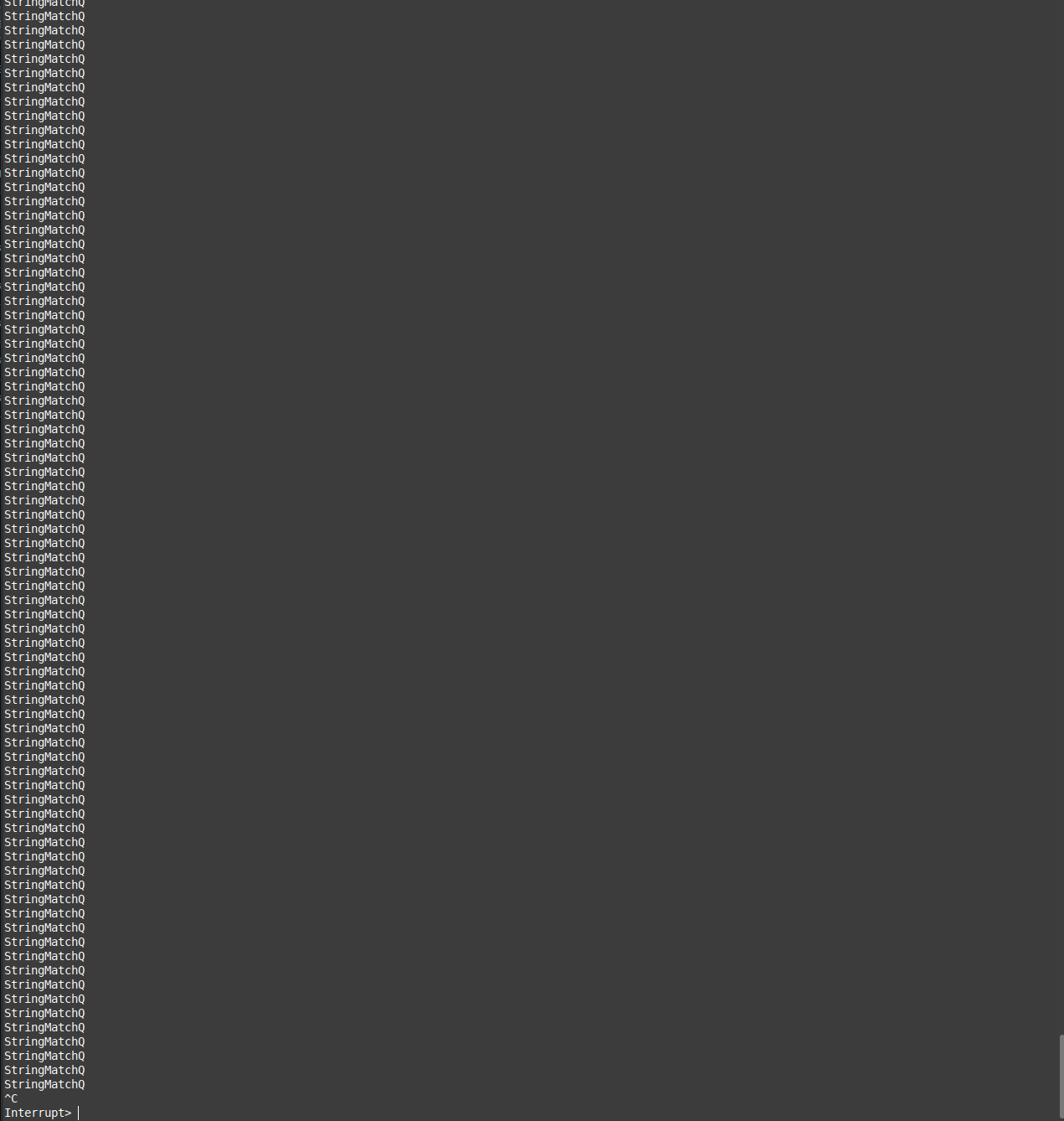
Clue for developers: If one runs this in terminal and traces the whole calculation ("Crtl-C" and then "t"), will see a million lines of StringMatchQ apperaing on the screen.
Closeing words:
I understand that Mathematica, as a for-profit company, must generate revenue. However, I sincerely believe their current business model, which appears to deprioritize fundamental mathematical fields, is far from ideal and may ultimately lead to its decline in popularity.
While I don't have access to Mathematica's specific revenue figures, it's clear that their income comes from both industry and academia. But these two sectors are not independent of each other. Engineers and other industry professionals typically first encounter Mathematica during their university years, where professors assign coursework requiring the use of this language. These professors choose Mathematica precisely because it's the tool they know best and use daily in their own work. This creates a natural stream of students learning Mathematica in academia, then carry that expertise into industry and convincing their boss to buy licenses.
While I acknowledge that machine learning and AI capabilities are undoubtedly part of the technological future, so are the fundamental functions that have always been Mathematica's strength: Factor, Expand, Series, Apart, DSolve, Integrate, FindNullVector just to name a few. I seriously doubt that Mathematica's most valuable part is its artificial intelligence features. The computational landscape extends far beyond AI; symbolic calculation, graph theory, finite field methods, numerical simulations and GPU computing are all have widespread adoption across numerous fields, both industry and academic.
To be clear, I'm not suggesting that Mathematica should abandon AI development or focus exclusively on traditional mathematical computation. Rather, I'm arguing for a balanced approach. If Mathematica fails to keep its core mathematical functions, the very features that attracted researchers in the first place, updated to meet contemporary challenges, it risks losing its academic user base. Once researchers migrate to alternative platforms that better serve their needs, the downstream effects are inevitable. The decline won't be sudden or dramatic; instead, it will manifest as a slow but steady erosion over years as competing languages gradually take over both research and industry.
The path forward seems clear to me; Mathematica must ALSO invest in keeping its fundamental mathematical capabilities at the cutting edge while simultaneously developing new features. Only by maintaining excellence in both traditional and emerging areas can they preserve their market position and ensure long-term profits.
 Attachments:


