Group Abstract Group Abstract

Message Boards Message Boards

0
|
80 Views
|
5 Replies
|
7 Total Likes
View groups...
Share
Share this post:

Visualizing derivative logic: chain rule decompositions vs. symbolic solvers

Posted 2 days ago

Hello Community,I’ve been exploring different ways to teach the "Chain Rule" to students who find the standard Leibniz notation $dy/dx = dy/du \cdot du/dx$ a bit abstract when applied to nested functions like $f(g(h(x)))$.While D[f[g[x]], x] in Wolfram Language gives the perfect result instantly, I’ve found that students often benefit from seeing a "Step Tree" or a "Decomposition Table" to understand which rule is being applied at which depth. I’ve been building a project to automate this specific pedagogical breakdown: Derivative Calculus Solver. It focuses on showing the intermediate "substitution" steps that occur before reaching the final simplified form.My Question: > When handling highly nested functions, do you find it more effective to teach the "Inside-Out" method (starting with the innermost function) or the "Outside-In" (the standard Power/Chain rule approach)?For example, in the following WL code, the result is clear, but the "logic path" can be interpreted in two ways:Code snippet(* A nested example for discussion *)

f[x_] := Cos[Log[x^2 + 1]]^3
D[f[x], x] // TraditionalForm

I’ve tried to align the logic on my site with the WolframAlpha["derivative of...", "Steps"] output, but I’m curious if the community has thoughts on how to better visualize "partial results" for students who get lost in the algebra. Looking forward to your insights!

5 Replies

I am a calculus teacher too, now retired, and I am glad to be useful. On YouTube I shared my introductory lecture to the derivative, made using Mathematica. It is in Italian, though.

POSTED BY: Gianluca Gorni

Gianluca, thank you for this! That is an incredibly elegant use of Framed and ReplaceRepeated (//.). It’s a very clean way to help students identify the "inner" function $g(x)$ without the visual overhead of a full tree. It’s interesting to see the contrast in approaches here. While I built

Derivative Calculus Solver

to focus on the step-by-step substitution logic (explicitly showing $u$ and $du/dx$), your method focuses on the spatial structure of the composition. I think combining these two—using your "Framing" method to identify the target and then a step-by-step solver to execute the differentiation—would be the ultimate way to prevent students from getting lost in nested functions. Thanks for sharing such a concise snippet!

Michael, thank you for such a detailed and insightful response! Your point about the "extreme elaborateness" of complex branching functions is a powerful argument for the Outside-In approach. You are absolutely right—once you introduce products or sums within the composition, like in your example $f(g(h(k)\cdot m(n+p(q))))$, the "inside" becomes a moving target. Starting from the outermost operator is the only way to maintain a consistent algorithmic path. I particularly like your use of color-coding to track the "active" differentiation layer. In developing

Derivative Calculus Solver

, I faced a similar challenge in UI design: how to show the "Inside" function clearly while the "Outside" is being processed. Inspired by the hybrid Leibniz/Differential method you mentioned ( $d(f(u)) = f'(u) du$), I structured my tool to explicitly define $u$ at each step. This seems to help students who struggle with the "bookkeeping" aspect of the chain rule that you highlighted. Your custom Wolfram code for the dt function is excellent. The way it recursively generates the "Step Tree" using ColorData is a brilliant pedagogical tool for the community. I will certainly be spending some time studying your to Univariate Power rules—that’s a very elegant way to handle Power[] objects for visualization. Thank you for sharing your 1981-to-present perspective; it’s rare to see such a clear bridge between the history of CAS and modern teaching methods!

Here's a representation of how I show my students. It's for strictly composite formulas, by which I mean functions of the form $f\circ g \circ \cdots \circ h$ or as a formula $f(g(\cdots h(x)))$. It won't deal with a formula like the following: $$f\left(g\bigl(h(k(l(x)))\cdot m(n(x)+p(q(r(x))))\bigr)\right) \tag{1}$$

The extreme elaborateness of $(1)$ is just to drive home why I wouldn't consider going "inside-out" with the chain rule. I suppose it's clear enough what to do on $\ln(\cos(e^x))$, but when the inside components involve combinations of sums, products, quotients, and compositions such as $\ln(\cos(x^2)+\sin(e^{3x})$, where do you start on the inside? At $x^2$ or $3x$? Or do you start in the middle with $\cos(x^2)+\sin(e^{3x}$ and work your way both up and down? How in the world could I ever explain the process to a group of students?

But mainly I go "outside-in", because that's how I was taught and that's all I have ever done. My first year in college in 1981, I was introduced to computational symbolic algebra in first-year math (via LISP). A couple of years later, I learned to write parsers, and I wrote a small CAS for fun. Programming the chain rule seemed natural to go outside-in. Yet another reason is that when you start substitution in integrals, the first examples generally involve substitutions where one lets $u$ be the inside of the outermost function of one the factors. Thus outside-in is a way to quickly identify probable substitutions. If one goes inside-out, several consecutive substitutions might be needed.

Finally, one calculus book I once used wrote the chain rule in a hybrid Leibniz way, $d(f(u)) = f'(u) \; du$, and the derivative rules for all the particular functions in the corresponding differential form like this: $d(\cos u)=(-\sin u) \; du$, etc. At the end of the process, you divide by $dx$ or whatever to get the derivative. It was meant to be used outside-in as follows: $${ d(\ln(\cos e^x)) ={1\over \cos e^x}\cdot d(\cos e^x) ={1\over \cos e^x}(-\sin e^x) \cdot d(e^x) ={-\sin e^x\over \cos e^x} e^x \;dx }$$ Then divide by $dx$.

In any case, I usually teach it outside-in with the derivative operator $d/dx$ instead of the differential operator as follows:

Chain rule on OP's example

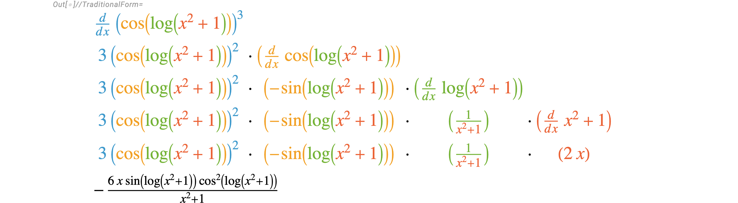
Of course, I don't write such colors on the board in class. (I usually underline the inside part to be differentiated on the outside per the chain rule, as a way to highlight it.)

Code dump

Fancy formatting needs fancy code unfortunately.

ClearAll[dt, dd, pow, exp, pp];
(* Univariate forms of Power[] *)
pow[k_]'[x_] := 
  If[k == 2, 2 x, k*pow[k - 1][x]]; (* power functions #^k& *)
exp[k_]'[x_] := Log[k]*exp[k][x]; (* exponential functions k^#& *)
toUnivariatePower = {sum_Plus :> sum, term_Times :> term, 
   Power[a_, b_] /; ! FreeQ[a, x] :> pow[b][a], 
   Power[a_, b_] /; ! FreeQ[b, x] :> exp[a][b]};
fromUnivariatePower = {pow[b_][a_] :> Power[a, b], 
   exp[a_][b_] :> Power[a, b]};
MakeBoxes[pow[k_][x_], form_] := 
  SuperscriptBox[RowBox[{"(", MakeBoxes[x, form], ")"}], 
   MakeBoxes[k, form]];
MakeBoxes[exp[k_][x_], form_] := MakeBoxes[Power[k, x], form];
(* Extra parentheses and the derivative operator (for output display) *)
MakeBoxes[pp[y : _. pow[_][_]], form_] :=(* don't parenthesize *)
  MakeBoxes[y, form]; 
MakeBoxes[pp[y_], form_] :=(* parenthesize *)
  RowBox[{"(", MakeBoxes[y, form], ")"}]; 
MakeBoxes[dd[y_], form_] :=(* derivative operator *)
  RowBox[{ (* choose "d" or "\[PartialD]" *)
    FractionBox["d", "d\[InvisibleSpace]x"],
    MakeBoxes[y, form]}]; 

dt[f_[x_], "Style", n_] := 
  Style[f[dt[x, "Style", n + 1]], ColorData[116][n]];
dt[y_, "Style", n_] := Style[y, ColorData[116][n]];
dt[y_] := TraditionalForm@Grid[
    Replace[
     Rest /@ dt[dt[murf = y //. toUnivariatePower, "Style", 1], {}]
     , row_List /; Length@row > 1 && FreeQ[row, SpanFromLeft] :>
      Replace[row, Style[x_, s_] :> Style[pp@x, s], 1], 1]
    , Alignment -> Automatic, Spacings -> {0, Automatic}];
dt[sf : Style[f_[x_], s__], 
   pre_] := {{Sequence @@ pre, " \[CenterDot] ", Style[dd[f[x]], s]},
   Sequence @@ dt[x, Join[pre, {" \[CenterDot] ", Style[f'[x], s]}]]};
dt[sy : Style[y_, s__], 
   pre_] := {{Sequence @@ pre, " \[CenterDot] ", Style[dd[y], s]},
   Sequence @@ dt[x, Join[pre, {"\[CenterDot]", Style[D[y, x], s]}]]};
dt[x, pre_] := {pre, {Null, 
    Item[Times @@ pre[[2 ;; ;; 2]] /. 
        RawBoxes -> (ReleaseHold@
            MakeExpression[#, TraditionalForm] &) /. 
       Style -> (# &) //. fromUnivariatePower, Alignment -> Left], 
    SpanFromLeft}};

(* Example shown above: *)
dt[Cos[Log[x^2 + 1]]^3]
POSTED BY: Michael Rogers

This is my little attempt to visualize the nested composition of functions:

func = Cos[Log[x^2 + 1]]^3;
func //. Cases[func, f_[g_] :> (f[g] :> f[Framed[g]]), All]
% //. Cases[%, f_^n_Integer /; f =!= x :> (f^n :> Framed[f]^n), All]
POSTED BY: Gianluca Gorni
Reply to this discussion
Community posts can be styled and formatted using the Markdown syntax.
Reply Preview
Attachments
Remove
or Discard