Message Boards Message Boards

0
|
12859 Views
|
2 Replies
|
2 Total Likes
View groups...
Share
Share this post:

Trying to simulate electric field lines from collection of point charges

Posted 10 years ago

So, I'm fairly new to Mathematica; sorry if this ends up being a very dumb question. I've been trying to simulate and plot electric field lines from point charges in Mathematica. The first resource I found is Wolfram's Electric Field Lines Due To A Collection of Point Charges, but I've been having trouble figuring out how one would incorporate more source charges. What I think I'm not quite understanding is the first lines of code defining the electric field - I don't understand how p and pp are being defined, or why it wouldn't work to simply add a third term along the lines of qi and so on. If anyone can offer any insight, I'd be very grateful.

 eeX = Compile[{{q, _Real, 1}, {pp, _Real, 2}, {p, _Real, 1}}, 
        Sum[{-((q[[i]] (p[[1]] - pp[[i, 1]]))/
((p[[1]] - pp[[i, 1]])^2 + (p[[2]] - pp[[i, 2]])^2)^(3/2)), 
-((q[[i]] (p[[2]] - pp[[i, 2]]))/
((p[[1]] - pp[[i, 1]])^2 + (p[[2]] - pp[[i, 2]])^2)^(3/2)),
 {i, Length[pp]}]]
POSTED BY: Amy Zimmerman
2 Replies

Hey Amy,

If you are given a point p in the plane and two sources pp = {source_1 , source_2}, the field at this point should be the vector sum of the fields induced by the two point sources. In your code, p is coordinate of a point you are interested and p[[1]] gives the x-coordinate of the point and so on. pp[[1,1]] gives the x-coordinate of source_1 and so on.

You do not have "tjhe third item" item because we are working on the 2D plane.

POSTED BY: Shenghui Yang
Posted 10 years ago

Hi Amy,

This is not their code, but may be a little easier to see into. It defines a function for the potential generated by a single charge, sums this for a list of charges, and then uses E = - grad V to get the field.

(* set the directory so we export plots it *)
SetDirectory[NotebookDirectory[]];

(* define a vector norm that does not use Abs *)
norm[a_] := Sqrt[a.a]

(* the potential at point (x,y) generated by charge q at (px,py) *)
ePot[{x_, y_}, {px_, py_, q_}] := q/norm[{x, y} - {px, py}]

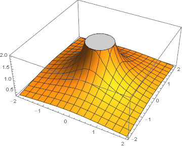
(* the potential of a point charge at the origin *)
p1 = Plot3D[ePot[{x, y}, {0, 0, 1}], {x, -2, 2}, {y, -2, 2}]

enter image description here

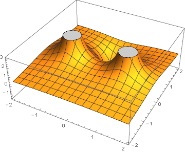
(* a list of charges *)
charges = {{-1, 0, 1}, {1, 0, 1}, {0, 1, -1}};

(* total potential at (x,y) from all the charges in a list *)
totPot = Total[ePot[{x, y}, #] & /@ charges];

(* the total potential *)
p2 = Plot3D[totPot, {x, -2, 2}, {y, -2, 2}]

enter image description here

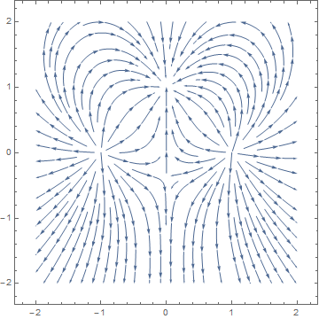
(* the field is minus the gradient of the potential *)
totField = -Grad[totPot, {x, y}];
p3 = StreamPlot[totField, {x, -2, 2}, {y, -2, 2}]

enter image description here

POSTED BY: David Keith
Reply to this discussion
Community posts can be styled and formatted using the Markdown syntax.
Reply Preview
Attachments
Remove
or Discard

Group Abstract Group Abstract