Would it be possible to do quantiles from a Pareto frontier? In other words, find points which pareto dominate x % of all the points?

The algorithm can be easily extended to 3D and higher dimensions, and I decided to illustrate that with an example. The 3D implementation is really easy using Mathematica's geometric computation functions (i) for derivation of rotation matrices and (ii) for region manipulation. (The latter are new in version 10.)

Let us first generate some data.

npoints = 10000;
data = {RandomReal[{0, 2 \[Pi]}, npoints], 
   RandomReal[{-\[Pi], \[Pi]}, npoints], 
   RandomVariate[PoissonDistribution[4.8], npoints]};
data = MapThread[#3*{Cos[#1] Cos[#2], Sin[#1] Cos[#2], Sin[#2]} &, data];

Let us plot the data:

Block[{qs = 12},
 qs = Map[Quantile[#, Range[0, 1, 1/(qs - 1)]] &, Transpose[data]];
 ListPointPlot3D[data, PlotRange -> All, PlotTheme -> "Detailed", 
  FaceGrids -> {{{0, 0, -1}, Most[qs]}, {{0, 1, 0}, 
     qs[[{1, 3}]]}, {{-1, 0, 0}, Rest[qs]}}, ImageSize -> 700]
 ]

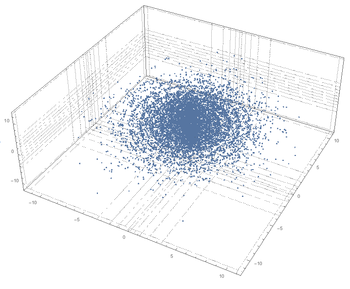
(On the plot the grid lines derived from the quantiles of x, y and z coordinates of the data set.)

Using the set of uniform angles:

nqs = 20;
dirs = N@Flatten[
    Table[{Cos[\[Theta]] Cos[\[Phi]], Sin[\[Theta]] Cos[\[Phi]], 
      Sin[\[Phi]]}, {\[Theta], 2 \[Pi]/(10 nqs), 2 \[Pi], 
      2 \[Pi]/nqs}, {\[Phi], -\[Pi], \[Pi], 2 \[Pi]/nqs}], 1];

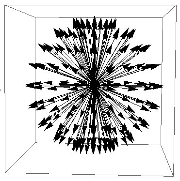
we can compute the quantiles of the z-coordinates in each direction:

rmats = RotationMatrix[{{1, 0, 0}, #}] & /@ dirs;

qs = {0.95};
qDirPoints = 
  Flatten[Map[Function[{m}, Quantile[(m.Transpose[data])[[3]], qs]], rmats]];

and produce the quantile envelope surface using ImplicitRegion and BoundaryDiscretizeRegion:

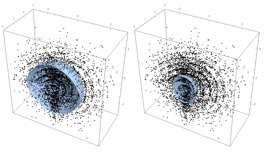
More details and examples of usage are given in my blog post: "Directional quantile envelopes in 3D" . Also, see the attached notebook.

Attachments: