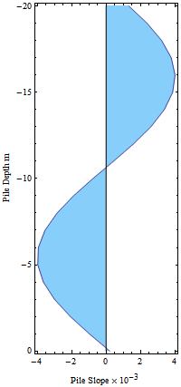
Okay, here is how I would draw it with my Presentations application. It's an example of working more with primitives than trying to modify a top-down design. ListLineDraw is like ListLinePlot except that it just returns the primitive graphics elements of the object being drawn without all the frame items. RotateOp is like Rotate except you can use it directly like a postfix operator without all the graphics to be rotated embedded in the middle. CustomTicks allows you to specify your own ticks and subticks. I used it here to reverse the y-axis. I also drew a line for the vertical Pile Slope axis. It could just be mixed in with the other primitives. No Epilog or Graphics level jumping.

<< Presentations`

f[x_] := 4 Sin[0.3 (x + 10 \[Degree])]
fdata = Table[{x, f[x]}, {x, -20, 0, 1}];

yticks = CustomTicks[-# &, {-20, 0, 5, 5}];
Draw2D[
 {{ListLineDraw[fdata,
     Filling -> Axis,
     FillingStyle -> ColorData["Legacy"]["LightSkyBlue"]],
    Line[{{-20, 0}, {0, 0}}]} // RotateOp[-\[Pi]/2, {0, 0}]},
 Frame -> True,
 FrameTicks -> {{yticks, yticks // NoTickLabels}, {Automatic, 
    Automatic}},
 FrameLabel -> {"Pile Slope \[Times] \!\(\*SuperscriptBox[\(10\), \
\(-3\)]\)", "Pile Depth m" },
 ImageSize -> 200]

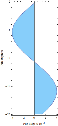
I realized that the above solution leaves out a needed reflection but that's easy to fix. Just add it after the rotation. One of the advantages of always dealing with primitives is that we can not only easily combine them - just draw one thing after another - but we can also easily manipulate them, individually if necessary.

Draw2D[
 {{ListLineDraw[fdata,
      Filling -> Axis,
      FillingStyle -> ColorData["Legacy"]["LightSkyBlue"]],
     Line[{{-20, 0}, {0, 0}}]} // RotateOp[-\[Pi]/2, {0, 0}] // 
   ReflectionMatrixOp[{0, 1}]},
 Frame -> True,
 FrameTicks -> Automatic,
 FrameLabel -> {"Pile Slope \[Times] \!\(\*SuperscriptBox[\(10\), \
\(-3\)]\)", "Pile Depth m" },
 ImageSize -> 200]

Hello Malcom, What is your goal here? Is it to learn how to make Mathematica create the plot, or is it to get the plot and move on to publishing it in a different medium?

If it is the later, I usually Export a plot without labels as an .svg (scalable vector graphics) and then import it into an svg editing program such as Inkscape (free) or Adobe illustrator (commercial). This is what I do if it is a one-off and in a hurry.

If the later, you might look at using rotated text to get what you want. There is an example of doing this in the Barchart documentation examples.

How would this be? You can place the left edge wherever you wish.

f[y_] := 3 + y Cos[y]
RegionPlot[-1 <= x <= f[y] && 0 <= y <= 4, {x, -2, 4}, {y, 0, 4},
 PlotRange -> {{-2, 4}, {-0.2, 4.5}},
 Frame -> True,
 ImageSize -> 300]

You can get the vertical lines on a plot by using

Exclusions -> None

If you have a "curve" that bounds the left axis and the upper horizontal boundry of the graph then you can fill to that. Here is an example:

Plot[
 {10 UnitStep[x], x}, {x, 0, 10}, Filling -> {1 -> {2}}, 
 PlotStyle -> {Directive[Opacity[0]], Directive[Red]}]

and

Plot[
 {100 UnitStep[x], x^2}, {x, 0, 10}, Filling -> {1 -> {2}}, 
 PlotStyle -> {Directive[Opacity[0]], Directive[Red]}]

You just have to get the coefficient of UnitStep correct for this to work.