Hi Torjus, I had a quick look, and there are a few ways of doing this. When you just plot the function like this:

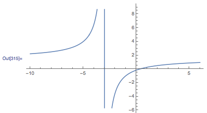
Plot[(3 x - 1)/(2 x + 6), {x, -10, 6}]

you get an output with the vertical asymptote:

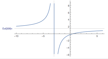
You can then just add another function to plot of 1.5, like this:

Plot[{(3 x - 1)/(2 x + 6), 1.5}, {x, -10, 6}]

This is fine, but if you want both asymptotes to be a different graphics primitive we will have to try something else. You can also use GridLines, though I find this a bit clunky:

Plot[(3 x - 1)/(2 x + 6), {x, -10, 6},GridLines->{{-3,0},{0,1.5}}]

OK, so now we have both asymptotes, but still the vertical one from the original plot. To stop this from showing up use Exclusions (an option in plot):

Plot[(3 x - 1)/(2 x + 6), {x, -10, 6},Exclusions->{x==-3},GridLines->{{-3,0},{0,1.5}}]

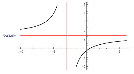
Another way, and my preferred method, is to use the option Epilog to add a Line primitive onto the plot. You can then style the asymptotes separately to make them more clear:

Plot[{(3 x - 1)/(2 x + 6), 1.5}, {x, -10, 6}, 
 PlotStyle -> {Black, Red}, Exclusions -> {x == -3}, 
 Epilog -> {Red, Line[{{-3, -100}, {-3, 100}}]}]

From here, you can use labelling options to add in your asymptote labels.

I hope this helps!

Nia Knibbs Vaughan