Abstract
We discuss classification as the data-mining technique in patterns recognition and supervised machine-learning. Comparison of classification to other data exploration methods is presented and the importance of this approach is further discussed. We demonstrate the machine-learning method in finance and show how credit risk categorisation can be easily achieved with classification technique.

Introduction
Searching for patterns in economic and financial data has a long history. One of the oldest approached explored by econometricians was the data arrangement into groups based on their similarities and differences. As computer resources improved there was a growth in the scope and availability of new computational methods. However, the greatest data analysis challenges are undoubtedly more recent. Advances in observational and collection methods have generated, and continue to generate enormous volumes of information that present significant storage, retrieval and analysis challenges.
The analytical tools that extract information from data can be placed into two broad and overlapping categories: (i) cluster and (ii) classification methods. Using these techniques, datasets can be classified according to a specific property by measurements indirectly related to the property of interest. An empirical relationship on the classification rule can be developed from a dataset for which the property of interest and the measurements are known. The classification rule can then be used to predict the property in samples that are not part of the original set.
In view of the above, we view classification as a data-mining technique that comes particularly helpful in finding patterns in the data that can dramatically reduce its dimensionality. It helps identifying class membership from prediction variables and identify features that either contribute or can be used to predict class membership.
Machine learning
Machine learning is a subset of artificial intelligence that incorporates a large number of statistical ideas and methods and uses algorithms that 'learn' from data. Learning is based around finding the relationship between a set of features in the data structure. Induction and deduction are two types of reasoning used in the learning process. Induction stems from the particular to the general and can be used to generate classification rules from examples by establishing 'cause-effect' relationships between existing facts. Deduction, on the other hand, is concerned with reasoning using existing knowledge. The requirement for previously acquired knowledge is one of the main differences between deduction and induction. Because deduction can be used to predict the consequences of events or to determine the prerequisite conditions for an observed event, it is at the heart of most expert systems.
Machine learning is primarily based on induction. Whilst this is natural consequence of the method itself, it leads to paternally two problems:
These difficulties are not restricted to machine learning. it is well known that relationships models based on regression should not be extrapolated beyond the limits of the original data. A good news, however, is that noise does not have consistent effects on machine learning algorithms; for example, neural networks, and instance-based methods all use 'distributed' representations This is important because distributed representations should be less susceptible to noise hence they have the potential to be more robust classifiers.
Supervised learning
Supervised learning applies to algorithms in which a 'teacher' continually assesses, or supervises, the classifier's performance during training by marking predictions as correct or incorrect. Naturally, this assumes that each case has a valid class label. Learning in this sense relates to the way in which a set of parameter values are adjusted to improve the classifiers' performance.
Unsupervised learning
On the other hand, in unsupervised learning there is no teacher and the classifier is left to find its own classes - known as clusters. The biggest benefits from an unsupervised classification are likely in knowledge-poor environments, particularly when there are large amounts of unlabeled data. As such clustering are viewed as a means of generating, rather than testing, hypotheses and related classifications.
Classification
Classification is the placing of objects into predefined groups. This type of process is also called 'pattern recognition'. Why? The set of samples for which the property of interest and measurements is known is called the training set. The set of measurements that describe each sample in the data set is called a pattern. The determination of the property of interest by assigning a sample to its respective category is called recognition, hence the term pattern recognition. . As such, it is a collection of methods for 'supervised learning'.
Clustering is related to classification. Both techniques place objects into groups or classes. The important difference is that the classes are not predefined in a cluster analysis. Instead objects are placed into 'natural' groups.Therefore, clustering algorithms are unsupervised.
When we deal with large sets of multidimensional data, we can apply standard methods such as PCA (principal component analysis) or clustering. Both techniques attempt to analyse data without directly using information about the class assignment of the samples. Although both are powerful methods for uncovering relationships in large multivariate data sets, they are not sufficient for developing a classification rule that can accurately predict the class-membership of an unknown sample.
Pattern recognition techniques fall into one of two categories:
Nonparametric discriminants,.such as neural networks, attempt to divide a data space into different regions. In the simplest case, that of a binary classifier, the data space is divided into two regions. Samples that share a common property (e.g. risk type) will be found on one side of the decision surface, whereas those samples comprising the other category will be found on the other side. Classification based on random or chance separation.can be a serious problem if the data set is not sample rich. Because economic datasets usually contain more variables than samples, similarity-based classifiers are generally preferred.
A basic assumption in similarity-base classification is that distances between points in the measurement space will be inversely related to their degree of similarity. Using a similarity-based classifier we can determine the class-membership of a sample by examining the class label of the data point closest to it in the measurement space.
Classification in Mathematica 10 can be efficiently performed with the Classify command which offers good degree of flexibility and classification method selection.
Classification techniques in Finance
Classification can be effectively used in the risk management and large dataset processing where group information is of particular interest.
Consider the following case: financial institution has large portfolio of loans to its clients. It wants to establish the method for assessing the quality of lending portfolio by linking the maturity and credit spread on each loan to internal rating categories. We apply the Classification method to analyse the portfolio and to assign each loan to the rating class. Finally we produce the classified loans status based on the rating group ping.
Training set definition
The financial institution can define the training set (the template for sample assignment) in the following way:
6 Rating categories: AAA,, AA, A, BBB, BB, B
3 maturity sets: 3 years / 5 years / 10 years
Credit spreads for each maturity / rating
trainset = {{3, 50} -> "AAA", {5, 70} -> "AAA", {10, 85} ->
    "AAA", {3, 85} -> "AA", {5, 145} -> "AA", {10, 200} ->
    "AA", {3, 120} -> "A", {5, 200} -> "A", {10, 260} ->
    "A", {3, 210} -> "BBB", {5, 300} -> "BBB", {10, 390} ->
    "BBB", {3, 290} -> "BB", {5, 370} -> "BB", {10, 440} ->
    "BB", {3, 360} -> "B", {5, 470} -> "B", {10, 550} -> "B"};
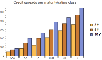
By isolating credit spreads, we can visualise the training set credit spreads levels below:
sprd = {{50, 70, 85}, {85, 145, 200}, {120, 200, 260}, {210, 300, 390}, {290, 370, 440}, {360, 470, 550}};
BarChart[sprd, ChartLegends -> {3 Y, 5 Y, 10 Y},
 PlotLabel -> Style["Credit spreads per maturity/rating class", 15],
 ChartLabels -> {{"AAA", "AA", "A", "BBB", "BB", "B"}, None}]
Setting the classifier
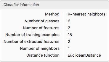
We use the training set defined above to set up the classifier based on similarity measure using k-nearest neighbor method
clsf = Classify[trainset, Method -> "NearestNeighbors"]

and obtain the information on the classifier
ClassifierInformation[clsf]
We can investigate the classifier further by obtaining additional Information:
ClassifierInformation[clsf, "MethodDescription"]

Classifier testing
We can test and validate the classifier with the <ClassifierMeasurements> command. For example, we can define the validation test set as follows:
vset = {{3, 46} -> "AAA", {5, 81} -> "AAA", {10, 92} -> "AAA", {3, 91} ->
    "AA", {5, 155} -> "AA", {10, 202} -> "AA", {3, 126} -> "A", {5, 215} ->
    "A", {10, 259} -> "A", {3, 219} -> "BBB", {5, 311} -> "BBB", {10, 399} ->
    "BBB", {3, 292} -> "BB", {5, 378} -> "BB", {10, 442} -> "BB", {3, 350} ->
    "B", {5, 460} -> "B", {10, 568} -> "B"};
Testing accuracy of the classifier
cm = ClassifierMeasurements[clsf, vset]
cm["Accuracy"]

1.
The classifier returns the correct class group ping for all categories with high precision.
Measuring F-Score
cm["FScore"]
<|"A" -> 1., "AA" -> 1., "AAA" -> 1., "B" -> 1., "BB" -> 1., "BBB" -> 1.|>
Generating Confusion matrix
cm["ConfusionMatrixPlot"]
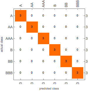
The matrix confirms that the classifier assigns the sample test data to the rating classes correctly. There are no overlaps in the assignment.
Applying classifier to the financial data
Applying classifier to the financial data
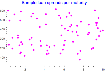
Having defined and tested the classifier, we can start applying it to the financial data. Let's assume that financial institution has 50,000 loans with remaining maturity / market spread information. The sample of the loan portfolio is shown below:
dat2 = Table[{RandomReal[10], RandomInteger[{70, 620}]}, {50000}];
Take[dat2, 75]
ListPlot[%, PlotStyle -> Magenta, PlotLabel -> Style["Sample loan spreads per maturity", Blue, 15]]
{{8.518356726448882,454},{9.144298651160256,608},{2.855364088031351,184},{6.0566791640110615,282},{1.5475654397289134,266},{2.6417875173168994,315},{4.966702524403626,231},{0.19793692995662404,605},{4.478200060877295,213},{9.292431559943076,294},{9.28184530814859,447},{4.204004132022266,234},{2.4319873689548466,296},{0.34979911441219613,499},{4.188999084728859,139},{9.94074933345011,392},{3.4739994419209292,429},{8.95426428111189,206},{8.554799166603996,367},{1.4762114253028358,498},{3.1821905760430784,520},{9.366754802446565,473},{1.6701704343156525,244},{1.376279011603522,232},{9.566319795447356,333},{0.8703633914472597,564},{6.71837887079888,452},{7.302098986957059,441},{2.6238815271294573,239},{1.5336733840535572,157},{1.4641136928541592,146},{0.6465197801125662,198},{1.222074695630404,315},{5.702826552095841,339},{6.731378893601473,552},{8.808804286652013,195},{0.6739420557112723,314},{6.378960901113356,393},{5.72547626395229,445},{9.460117372811034,417},{7.24575011914737,376},{3.542651788089211,280},{9.266105852374011,473},{0.07409813721899816,238},{6.042215952909746,412},{4.264033025081259,176},{2.6031280721072108,541},{0.30796996377340946,240},{7.365932988439827,339},{6.898537558573874,269},{7.588189071934799,80},{7.64691230466779,173},{4.097033804059016,456},{7.365705637020458,141},{6.499421726202534,578},{8.431948572861224,351},{6.241593889798619,540},{5.458576916155449,551},{1.2166050064107576,340},{5.5963915988722395,146},{5.958260855340793,235},{1.5241468668957854,595},{9.71283120935691,382},{3.604748368454281,226},{6.595824594015976,431},{5.125769853255001,619},{1.9166780841799138,121},{9.506908583817971,526},{2.793767635980249,574},{5.83433511143844,186},{7.708892750256794,484},{4.099308138686737,568},{5.6066580959611265,527},{4.377895268594408,146},{6.840495656634236`,380}}
We apply the classifier to the spread data:
clsloans = clsf[#] & /@ dat2;
and group the results into rating classes
rtdgroup = {"AAA", "AA", "A", "BBB", "BB", "B"};
rtdfreq = Table[Count[clsloans, i], {i, rtdgroup}]
BarChart[rtdfreq, ChartStyle -> "Rainbow", ChartLegends -> rtdgroup,
 ChartLabels -> rtdgroup, LabelingFunction -> Above,
 PlotLabel -> Style["Rating classification of 50,000 loans portfolio", Blue, 15]]
{720, 9003, 6481, 8878, 6867, 18051}
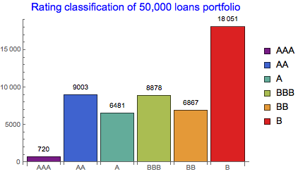
We can see that the largest proportion of loans falls into B-rated category and the smallest to the AAA category. This is naturally expected. Further aggregation of the classified results can be done on Investment grade (>BB) and Non-Investment grade scale:
{Total[rtdfreq] - Total[Take[rtdfreq, -2]], Total[Take[rtdfreq, -2]]};
BarChart[%, ChartStyle -> "Pastel", ChartLegends -> {"IG Loans", "Non-IG Loans"},
 LabelingFunction -> Above, PlotLabel -> Style["Investment grade / Non-investment grade split", Blue, 15]]
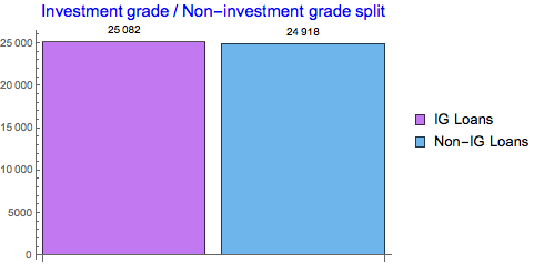
We can see equal split between IG and non-IG loans.
Dynamic update of the portfolio
The set-up classifier can work with dynamically changing portfolio. For example, we can add 100 new loans to the existing portfolio and visualise the result:
newport=Table[Count[Join[clsloans,clsf[#]&/@
    Table[{RandomReal[10],RandomInteger[{70,620}]},{50}]],i],{i,rtdgroup}];
{BarChart[rtdfreq,ChartStyle->"Rainbow",ChartLegends->rtdgroup,ChartLabels->rtdgroup,
    LabelingFunction->Above,PlotLabel->Style["Existing portfolio",Blue,15],ImageSize->290],
BarChart[newport,ChartStyle->"TemperatureMap",ChartLegends->rtdgroup,ChartLabels->rtdgroup,
    LabelingFunction->Above,PlotLabel->Style["Portfolio with added 100 new assets",Blue,15],ImageSize->290]}

We can also simulate the generation of new load assets and see how they are dynamically classified using the classification defined on the training set.
Manipulate[BarChart[Table[Count[clsf[#] & /@
     Table[{RandomReal[10], RandomInteger[{70, 620}]}, {\[Alpha]}], i],
    {i, rtdgroup}], ChartStyle -> "DarkRainbow", ChartLegends -> rtdgroup,
  ChartLabels -> rtdgroup, LabelingFunction -> Above,
  PlotLabel -> Style["Classified new loans in the portfolio", Blue, 15]],
    {{\[Alpha], 10, "Nb of new loans"}, 0, 100, 1}]
Review of the classification algorithms
We can further investigate the behaviour of the classification algorithm by looking at the probability assignment boundaries for each class. We select the 5 year horizon for presentation purposes and pick the IG group:
{Plot[clsf[{5,x},{"Probability","AAA"}],{x,0,150},PlotStyle->Blue,Filling->Axis,PlotLabel->Style["AAA Rated",13]],
Plot[clsf[{5,x},{"Probability","AA"}],{x,0,240},PlotStyle->Magenta,Filling->Axis,PlotLabel->Style["AA Rated",13]],
Plot[clsf[{5,x},{"Probability","A"}],{x,0,300},PlotStyle->Green,Filling->Axis,PlotLabel->Style["A Rated",13]],
Plot[clsf[{5,x},{"Probability","BBB"}],{x,0,400},PlotStyle->Orange,Filling->Axis,PlotLabel->Style["BBB Rated",13]]}

This 'digital-alike' behaviour of the NearestNeighbors algorithm is the one we actually desire in the probabilistic setting. This ensures limited overlap / spillage between the class boundaries.
When we selected other classification algorithms, the result can be quite different. This is demonstrated below:
Random Forest classification
clsfRF = Classify[trainset, Method -> "RandomForest"];

method=clsfRF;
{Plot[method[{5,x},{"Probability","AAA"}],{x,0,150},PlotStyle->Blue,Filling->Axis,PlotLabel->Style["AAA Rated",13]],
Plot[method[{5,x},{"Probability","AA"}],{x,0,240},PlotStyle->Magenta,Filling->Axis,PlotLabel->Style["AA Rated",13]],
Plot[method[{5,x},{"Probability","A"}],{x,0,300},PlotStyle->Green,Filling->Axis,PlotLabel->Style["A Rated",13]],
Plot[method[{5,x},{"Probability","BBB"}],{x,0,400},PlotStyle->Orange,Filling->Axis,PlotLabel->Style["BBB Rated",13]]}

Neural Networks classification
clsfNN = Classify[trainset, Method -> "NeuralNetwork"];

method=clsfNN;
{Plot[method[{5,x},{"Probability","AAA"}],{x,0,150},PlotStyle->Blue,Filling->Axis,PlotLabel->Style["AAA Rated",13]],
Plot[method[{5,x},{"Probability","AA"}],{x,0,240},PlotStyle->Magenta,Filling->Axis,PlotLabel->Style["AA Rated",13]],
Plot[method[{5,x},{"Probability","A"}],{x,0,300},PlotStyle->Green,Filling->Axis,PlotLabel->Style["A Rated",13]],
Plot[method[{5,x},{"Probability","BBB"}],{x,0,400},PlotStyle->Orange,Filling->Axis,PlotLabel->Style["BBB Rated",13]]}

Support Vector Machine
clsfSVM = Classify[trainset, Method -> "SupportVectorMachine"];

method=clsfSVM;
{Plot[method[{5,x},{"Probability","AAA"}],{x,0,150},PlotStyle->Blue,Filling->Axis,PlotLabel->Style["AAA Rated",13]],
Plot[method[{5,x},{"Probability","AA"}],{x,0,240},PlotStyle->Magenta,Filling->Axis,PlotLabel->Style["AA Rated",13]],
Plot[method[{5,x},{"Probability","A"}],{x,0,300},PlotStyle->Green,Filling->Axis,PlotLabel->Style["A Rated",13]],
Plot[method[{5,x},{"Probability","BBB"}],{x,0,400},PlotStyle->Orange,Filling->Axis,PlotLabel->Style["BBB Rated",13]]}
We observe very different classification schemes when the algorithm changes from NearestNeighbors to other alternatives. Whilst RandomForest generates patchy classification pattern, artificial NeuralNetworks or SupportVectorMachine produce smooth probabilistic curves. However, such smoothness may be less desirable in the rating assignment context. This is demonstrated below:
Example: we want to test 4.5 years maturity and 110 bp spread.
NearestNeighbors sees this as A-rated asset given the proximity measure
clsf[{4.5, 110}, "Probabilities"]
<|"A" -> 0.722222, "AA" -> 0.0555556, "AAA" -> 0.0555556, "B" -> 0.0555556, "BB" -> 0.0555556, "BBB" -> 0.0555556|>
RandomForest generates multiple set of statistically important probabilities with less clear-cut assignment
clsfRF[{4.5, 110}, "Probabilities"]
<|"A" -> 0.254235, "AA" -> 0.212853, "AAA" -> 0.167341, "B" -> 0.119395, "BB" -> 0.110873, "BBB" -> 0.135303|>
NeuralNetworks sees this spread as primarily BBB-rates asset, but there is still strong support for A-rating as well
clsfNN[{4.5, 110}, "Probabilities"]
<|"A" -> 0.316899, "AA" -> 0.0229639, "AAA" -> 0.00319862, "B" -> 0.00256616, "BB" -> 0.0709275, "BBB" -> 0.583445|>
SupportVectorMachine provides similarly a set of statistically significant probabilities - seeing this as A-rates asset with other still being significant for quick conclusion
clsfSVM[{4.5, 110}, "Probabilities"]
<|"A" -> 0.415746, "AA" -> 0.210153, "AAA" -> 0.105478, "B" -> 0.0119384, "BB" -> 0.0444652, "BBB" -> 0.212219|>
The NearestNeighbors classification scheme produces the most consistent result in terms of data association with the rating class. In the context of this particular assignment this is the preferred method.
Conclusion
Classification is a powerful method for data organisation and dimensionality reduction in supervised machine learning. It is particularly useful when data has to be organised into class structure or given certain association with structural hierarchy. This is ideal for finding patterns in large datasets.
Classification is well-suited technique for financial data analysis. This was demonstrated on the credit rating case where simple implementation led to a power full and robust scheme that was able to classify large portfolios with real-time updates. As such, classification is therefore essential for prudent risk management.