Message Boards Message Boards

0
|
8476 Views
|
6 Replies
|
0 Total Likes
View groups...
Share
Share this post:

Nonlinearmodel Fit, Help needed!

Posted 9 years ago

Hi, I want to fit a sinc function to the data, you can find in the attachment. This is what I've done so far:

In[2]:= a245temp = Import["Desktop/A245_temp.txt", "Table"];

In[95]:= ListPlot[a245temp, PlotRange -> All, Frame -> {True}] 

enter image description here

In[51]:= model = P*Sin[a (t - T)]^2/(a (t - T)) + m*t + Q

Out[51]= Q + m t + (P Sin[a (t - T)]^2)/(a (t - T))

In[92]:= SincFit = 
 NonlinearModelFit[a245temp, 
   model, {{P, 40}, {a, .6}, T, {m, -0.012}, {Q, 1.8}}, t] // Normal

Out[92]= -51.8742 + 1.48008 t + (
 580.662 Sin[0.448411 (2.70343 + t)]^2)/(2.70343 + t)

But the fit does not work, as you can see here:

In[94]:= Plot[SincFit, {t, 27, 40}]

enter image description here

Can someone hepl me please?

Attachments:
POSTED BY: Sarmed Hussain
6 Replies

Jim, Good question! I don't know the details of how the data was obtained, but you get a Sinc function if you Fourier transform a rectangle: rectangle function. However if the rectangle is somehow modified by some smoothing function, the resulting transform has a main lobe that is typically wider but has smaller side lobes. Also as this seems to be a measurement, you have background noise that can drown out the lower lobes, which is defined by the signal to noise ratio.

I agree, from the first post I too thought we are dealing with something like a Gaussian distribution, but obviously from the type of measurement a Sinc function is expected.

POSTED BY: Kay Herbert
Posted 9 years ago

Hey, thank you very much. That's perfect! Yes there was indeed an error in my formula, i wanted the sinc^2-function.

POSTED BY: Sarmed Hussain
Posted 9 years ago

I confess that I didn't know of the Sinc function and incorrectly assumed it was a misspelling. Sorry about that.

However, given that the data does not share the characteristics of the fitted curve (the oscillations on either side of the peak are larger than what is displayed in the data), does this give evidence that the "expected" curve form shouldn't be expected or that the measurement instrument doesn't pick up the expected oscillations? Or something else?

Yes, this is not a Mathematica question but I ask because this is part of the complete process of fitting curves to data. FindFit uses least-squares for which inferences about the parameters and predictions depends on or assumes independent random errors of constant variance. It appears that the residuals are highly correlated and/or the curve form is not adequate to describe the observed data.

POSTED BY: Jim Baldwin

Hi, This is how I would solve it:

In[270]:= Clear["Global`*"]

In[271]:= 
data = {{27, 2.2}, {27.2, 2.2}, {27.4, 2.3}, {27.6, 2.3}, {27.8, 
    2.2}, {28, 2.2}, {28.2, 2.3}, {28.4, 2.2}, {28.6, 2.2}, {28.8, 
    2.3}, {29, 2.2}, {29.2, 2.2}, {29.4, 2.3}, {29.6, 2.2}, {29.8, 
    2.3}, {30, 2.3}, {30.2, 2.3}, {30.4, 2.3}, {30.6, 2.3}, {30.8, 
    2.3}, {31, 2.3}, {31.2, 2.3}, {31.4, 2.3}, {31.6, 2.3}, {31.8, 
    2.3}, {32, 2.3}, {32.2, 2.3}, {32.4, 2.3}, {32.6, 2.3}, {32.8, 
    2.4}, {33, 2.4}, {33.2, 2.4}, {33.4, 2.4}, {33.6, 2.5}, {33.8, 
    2.6}, {34, 2.7}, {34.2, 2.7}, {34.4, 2.8}, {34.6, 3.5}, {34.8, 
    5.1}, {35, 10.3}, {35.2, 15.4}, {35.4, 21.1}, {35.6, 29.1}, {35.8,
     35.6}, {36, 38.4}, {36.2, 37.5}, {36.4, 32.8}, {36.6, 
    25.5}, {36.8, 17.5}, {37, 10.9}, {37.2, 6.4}, {37.4, 3.8}, {37.6, 
    2.8}, {37.8, 2.7}, {38, 2.9}, {38.2, 2.8}, {38.4, 2.7}, {38.6, 
    2.4}, {38.8, 2.3}, {39, 2.3}, {39.2, 2.4}, {39.4, 2.4}, {39.6, 
    2.4}, {39.8, 2.4}, {40, 2.3}};

In[272]:= \
(*pd=ListLogPlot[data,PlotStyle\[Rule]Red,PlotTheme\[Rule]"Detailed"]*)

In[273]:= nlm = 
 FindFit[data, pp (Sinc[a x - tt])^2 + q, {a, pp, tt, q, m}, x, 
  Method -> NMinimize]

Out[273]= {a -> -1.9653, pp -> 35.9368, tt -> -70.833, q -> 2.05044, 
 m -> -35.6927}

In[274]:= fitx[x_] = pp (Sinc[a x - tt])^2 + q /. %

Out[274]= 2.05044 + 35.9368 Sinc[70.833 - 1.9653 x]^2

In[275]:= (*fitp=LogPlot[fitx[x],{x,27,40},PlotStyle\[Rule]Green]*)

In[276]:= (*Show[pd,fitp]*)

I modified your equation took out the "m x" term and I used Sinc^2 instead Sin^2/x (not the same as Sin^2/x^2) not sure if you wanted that. "Method -> NMinimize" does the trick for this kind of fit. this is what I get:

curve fit

POSTED BY: Kay Herbert
Posted 9 years ago

Hey Jim, thank you for your reply. I'm sry but i didn't describe my problem properly. The data is from a measurement of the power of a laser as a function of the temperature of a crystal. The expected dependency is the sinc-function, i used for my fit-model. I wanted to show something like this:

enter image description here

This is done with gnu-plot. I wanted to use mathematica to get a similar result.

Thank you!

POSTED BY: Sarmed Hussain
Posted 9 years ago

NonlinearModelFit is probably working just fine. It's your model using a sine wave that's the problem. While the points show a definite peak that isn't the shape of a sine wave (which has a peak and a trough and repeats) although if you restricted your fit of a sine to about 35 to 37, you might do better.

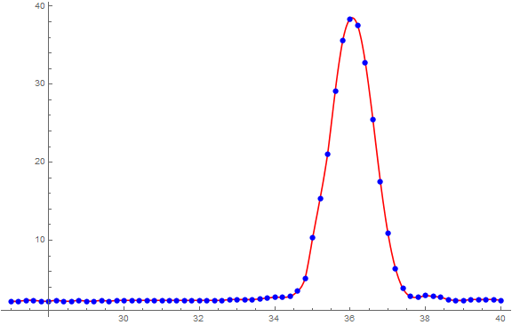
If you're mainly interested in approximating the curve (in Mathematica and not outside of Mathematica), then I recommend using the Interpolation function:

data = {{27, 2.2}, {27.2, 2.2}, {27.4, 2.3}, {27.6, 2.3}, {27.8, 2.2}, {28, 2.2}, {28.2, 2.3}, {28.4, 2.2}, {28.6, 2.2},
   {28.8, 2.3}, {29, 2.2}, {29.2, 2.2}, {29.4, 2.3}, {29.6, 2.2}, {29.8, 2.3}, {30, 2.3}, {30.2, 2.3}, {30.4, 2.3}, 
   {30.6, 2.3}, {30.8, 2.3}, {31, 2.3}, {31.2, 2.3}, {31.4, 2.3}, {31.6, 2.3}, {31.8, 2.3}, {32, 2.3}, {32.2, 2.3}, {32.4, 2.3},
   {32.6, 2.3}, {32.8, 2.4}, {33, 2.4}, {33.2, 2.4}, {33.4, 2.4}, {33.6, 2.5}, {33.8, 2.6}, {34, 2.7}, {34.2, 2.7}, {34.4, 2.8},
   {34.6, 3.5}, {34.8, 5.1}, {35, 10.3}, {35.2, 15.4}, {35.4, 21.1}, {35.6, 29.1}, {35.8, 35.6}, {36, 38.4}, {36.2, 37.5},
   {36.4, 32.8}, {36.6, 25.5}, {36.8, 17.5}, {37, 10.9}, {37.2, 6.4}, {37.4, 3.8}, {37.6, 2.8}, {37.8, 2.7}, {38, 2.9}, 
   {38.2, 2.8}, {38.4, 2.7}, {38.6, 2.4}, {38.8, 2.3}, {39, 2.3}, {39.2, 2.4}, {39.4, 2.4}, {39.6, 2.4}, {39.8, 2.4}, {40, 2.3}};
f = Interpolation[data];
Plot[f[x], {x, 27, 40}, PlotStyle -> Red, PlotRange -> Full];pPoints = ListPlot[data, PlotRange -> Full, PlotStyle -> Blue];
Show[{pInterpolation, pPoints}]

Interpolation function

But if you need a curve form with parameters to estimate so that you can use the predictions outside of Mathematica (and for which you can decide visually if the fit is good enough), then you might want to try something like

pNormalCurve = 
  Plot[2.1 + 55 PDF[NormalDistribution[36.05, 0.6], x], {x, 27, 40}, 
   PlotRange -> Full, PlotStyle -> {Thickness[0.02], LightGray}];
Show[{pNormalCurve, pInterpolation, pPoints}, ImageSize -> Large]

Normal curve fit

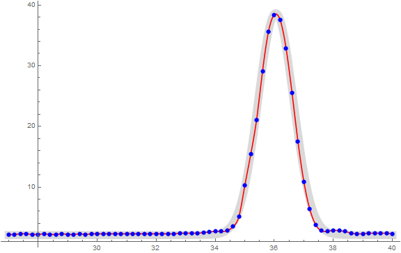
where the thick gray line is the normal curve fit. (I just did this by eye but you can use NonlinearModelFit also.)

If you need so say something about the parameters (i.e., measures of precision) and/or prediction errors, then something appropriate (in my opinion) depends on how the data is generated, if there will be multiple data sets which a need to compare parameters, how the residuals look, etc.

POSTED BY: Jim Baldwin
Reply to this discussion
Community posts can be styled and formatted using the Markdown syntax.
Reply Preview
Attachments
Remove
or Discard

Group Abstract Group Abstract