Since there is a parameter (It is not very clear what this parameter is but, I presume, like David, it is the initial condition y[x,0] (let it be alpha): In this case, ParametricNDSolve is a good choice

In[236]:= Clear[\[Alpha], sol, y]
a = 100; T = 60000; L = \[Pi];
sol = ParametricNDSolve[{I \!\(
\*SubscriptBox[\(\[PartialD]\), \(t\)]\(y[x, t]\)\) + .0004 \!\(
\*SubscriptBox[\(\[PartialD]\), \(x, x\)]\(y[x, t]\)\) == 0, 
    y[-a, t] == y[a, t], 
    y[x, 0] == 
     Piecewise[{{0, x < -(L/2)}, {0, 
        x > L/2}, {Sqrt[2/L] \[Alpha] Cos[x], -(L/2) <= x <= L/2}}]}, 
   y, {x, -a, a}, {t, 0, T}, {\[Alpha]}];
y /. sol
y[.1] /. sol
%[0., 0.5]

Out[239]= ParametricFunction[ <> ]

Out[240]= InterpolatingFunction[{{\[Ellipsis], -100., 
   100., \[Ellipsis]}, {0., 60000.}}, <>]

Out[241]= 0.0797883 - 5.73532*10^-7 I

and the Plot3D is really affected by the value of alpha as can be seen with a Manipulate:

Manipulate[
 Quiet@Plot3D[
   Evaluate[Abs[y[\[Alpha]][x, t]] /. sol], {x, -100, 100}, {t, -3.5, 
    3.5}, 
    PlotRange -> All, PlotPoints -> 50], {{\[Alpha], 1.57}, -5, 
  10, .01, Appearance -> "Labeled"}, SynchronousUpdating -> False]

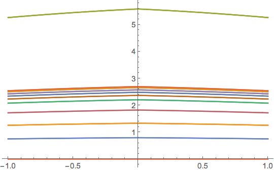
![][1] The effect of alpha can also be seen from the following plot:

Plot[Evaluate[
  Table[Abs[y[\[Alpha]][x, .95] /. sol], {\[Alpha], -10, 
    10}]], {x, -1, 1}]

sin = ClearAll
a = 50
T = 60000
L = \[Pi]
NDSolve[{I*\!\(
\*SubscriptBox[\(\[PartialD]\), \(t\)]\(y[x, t]\)\) + .0004*\!\(
\*SubscriptBox[\(\[PartialD]\), \(x, x\)]\(y[x, t]\)\) == 0, 
  y[-a, t] == y[a, t], 
  y[x, 0] == 
   Piecewise[{{0, x < -L/2}, {0, 
      x > L/2}, {Sqrt[2/L] Cos[x], -L/2 <= x <= L/2}}]}, y, {x, -a, 
  a}, {t, 0, T}]
Plot3D[Evaluate[Abs[y[x, t]] /. %], {x, -a, a}, {t, 0, T}, 
 PlotRange -> All, PlotPoints -> 200, MaxRecursion -> 2]

Sorry about that.