Message Boards Message Boards

[JAM] CellularAutomaton Code Jam Wolfram Summer School 2015

Posted 10 years ago

Wolfram Science Summer School and Wolfram Innovation Summer School are happening now in Boston at Bentley University. The goal of this Code Jam is to post interesting code snippets that fit the Wolfram Language functionality described in detail below. By "interesting" I mean simple programs that generate complex patterns. We will be jamming with our students, but everyone is welcome to join. Let's have some fun!

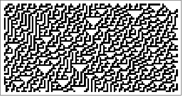
In this Code Jam we will take a look at the CellularAutomaton (CA) function and its syntax for rules defined as functions. This may sound a bit confusing, so let's take a look at some examples. First, if you haven't yet, you have to make yourself familiar with the CellularAutomaton function. The most well known cases are integer Wolfram indexes for CA rules, for instance for the celebrated rule 30:

ArrayPlot[CellularAutomaton[30, RandomInteger[1, 100], 50]]
enter image description here

But CellularAutomaton can take a function as a rule. Below are some examples. Use an arbitrary symbolic function f as the rule to apply to range-1 neighbors:

CellularAutomaton[{f[#] &, {}, 1}, {a, b, c}, 1]

{{a, b, c}, {f[{c, a, b}], f[{a, b, c}], f[{b, c, a}]}}

Set up a "Pascal's triangle cellular automaton":

CellularAutomaton[{f[#] &, {}, 1/2}, {a, b, c}, 1]

{{a, b, c}, {f[{c, a}], f[{a, b}], f[{b, c}]}}

CellularAutomaton[{Total[#] &, {}, 1/2}, {{1}, 0}, 3] 

{{1, 0, 0, 0}, {1, 1, 0, 0}, {1, 2, 1, 0}, {1, 3, 3, 1}}

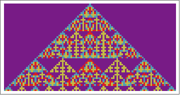
Additive cellular automaton modulo 4:

ArrayPlot[
 CellularAutomaton[{Mod[Total[#], 4] &, {}, 1}, {{1}, 0}, 50], 
 ColorFunction -> "Rainbow"]
enter image description here

The second argument to the function is the step number:

CellularAutomaton[{f[#1, #2] &, {}, 1}, {a, b, c}, 1]

{{a, b, c}, {f[{c, a, b}, 1], f[{a, b, c}, 1], f[{b, c, a}, 1]}}

CellularAutomaton[{f, {}, 1}, {a, b, c}, 1]

{{a, b, c}, {f[{c, a, b}, 1], f[{a, b, c}, 1], f[{b, c, a}, 1]}}

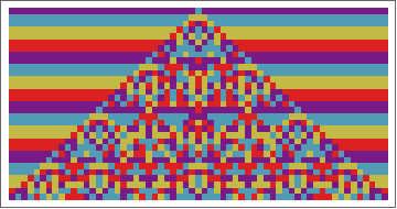
Change the rule at successive steps; #2 gives the step number:

ArrayPlot[
 CellularAutomaton[{Mod[Total[#] + #2, 4] &, {}, 1}, {{1}, 0}, 30], 
 ColorFunction -> "Rainbow"]
enter image description here

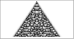
Use continuous values for cells:

ArrayPlot[CellularAutomaton[{Mod[Total[#]/2, 1] &, {}, 1}, {{1}, 0}, 50]]
enter image description here

Manipulate[
 ArrayPlot[
  CellularAutomaton[{Mod[s Total[#], 1] &, {}, 2}, {{1}, 0}, 50],
  ColorFunction -> "Rainbow", PixelConstrained -> 3]
 , {s, .01, .99}]
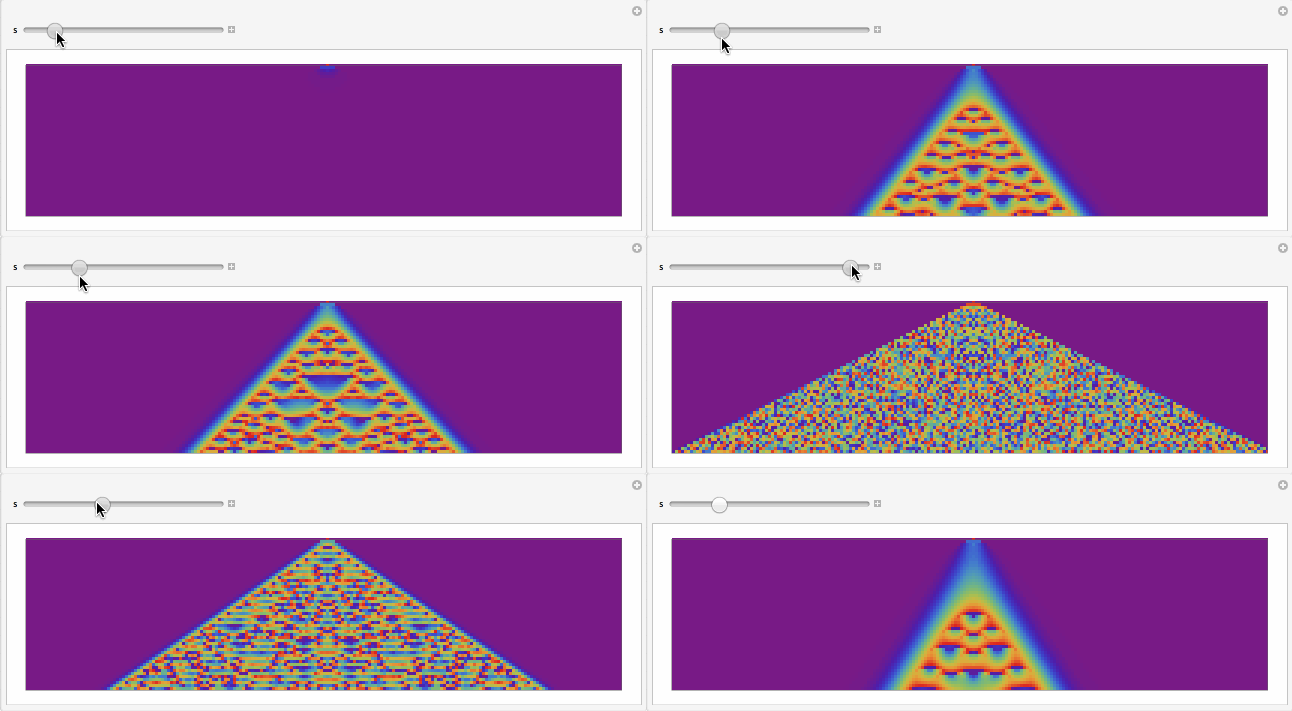
enter image description here

Try different functions and different initial conditions. They can be strings, numbers, graphics or expressions. Try ArrayPlot but also try other visualization tools like Grid. Try them out. Post code, images, and text comments. You can also comment on other people's code.

POSTED BY: Vitaliy Kaurov
46 Replies

enter image description here -- you have earned Featured Contributor Badge enter image description here Your exceptional post has been selected for our editorial column Staff Picks http://wolfr.am/StaffPicks and Your Profile is now distinguished by a Featured Contributor Badge and is displayed on the Featured Contributor Board. Thank you!

POSTED BY: EDITORIAL BOARD

i've compared the two forest fire programs, MySmokey and smokeyTheBear.

please excuse any formatting problems. doing 'copy and paste' from a notebook into this area causes a variety of problems (btw - the often-stated claim that most programs written in an early version of Mathematica run without difficulty in a later version of Matematica is simply untrue. even doing a simple 'copy and paste' of cells from a notebook created in an early version of Mathematica into a notebook in a later versions of Matematica is sometimes problematic.


In[1]:= Clear[MySmokey] MySmokey[nInteger (units), p (plant probability), f_ (fire probability), m_Integer (steps)] := With[{fcomp = Compile[{rand}, Evaluate[Floor[2 + f - rand]]], pcomp = Compile[{rand}, Evaluate[Floor[1 + p - rand]]]}, Module[{forestPreserve, forestIgnite, spreadFire, treeGrowIgnite}, forestPreserve = Table[Random[Integer], {n}]; SetAttributes[treeGrowIgnite, Listable]; treeGrowIgnite[0] := pcomp[Random[]]; treeGrowIgnite[1] := fcomp[Random[]]; forestIgnite[{path?(# === 1 &), 2, rem, 1}] := {spreadFire[path, 2], spreadFire[rem, 2]} /. 2 -> 0; forestIgnite[{1, rem, 2, path?(# === 1 &)}] := {spreadFire[2, rem], spreadFire[2, path]} /. 2 -> 0; forestIgnite[{rem__}] := {spreadFire[rem]} /. 2 -> 0; spreadFire[l, 2, 1, r] := Sequence[spreadFire[l, 2], spreadFire[2, r]]; spreadFire[l, 1, 2, r] := Sequence[spreadFire[l, 2], spreadFire[2, r]]; spreadFire[rem__] := rem; (Stopping criterion) NestList[forestIgnite[treeGrowIgnite[#]] &, forestPreserve, m]]]

In[3]:= Timing[MySmokey[100, 0.3, 0.2, 999];]

Out[3]= {0.252269, Null}


In[4]:= Clear[smokeyTheBear] smokeyTheBear[n, p, f, m] := Module[{}, forestPreserve = Table[Random[Integer], {n}]; pyro = (treeGrowIgnite = # /. {0 :> Floor[1 + p - Random[]], 1 :> Floor[2 + f - Random[]]}; forestIgnite = treeGrowIgnite //. {{2, c, 1} -> {2, c, 2}, {1, c, 2} -> {2, c, 2}, {a, 2, 1, b} -> {a, 2, 2, b}, {a, 1, 2, b} -> {a, 2, 2, b}}; forestIgnite /. 2 -> 0) &; NestList[pyro, forestPreserve, m]]


In[6]:= Timing[smokeyTheBear[100, 0.3, 0.2, 999];]

Out[6]= {0.386244, Null}

In[7]:= (SeedRandom[6]; smokeyTheBear[100, 0.3, 0.2, 0]) == (SeedRandom[6]; MySmokey[100, 0.3, 0.2, 0])

Out[7]= True

In[8]:= (SeedRandom[6]; smokeyTheBear[100, 0.3, 0.2, 1]) == (SeedRandom[6]; MySmokey[100, 0.3, 0.2, 1])

Out[8]= True

In[9]:= (SeedRandom[6]; smokeyTheBear[100, 0.3, 0.2, 25]) == (SeedRandom[6]; MySmokey[100, 0.3, 0.2, 25])

Out[9]= True

In[10]:= (SeedRandom[6]; smokeyTheBear[100, 0.3, 0.2, 26]) == (SeedRandom[6]; MySmokey[100, 0.3, 0.2, 26])

Out[10]= True

In[11]:= (SeedRandom[6]; smokeyTheBear[100, 0.3, 0.2, 27]) == (SeedRandom[6]; MySmokey[100, 0.3, 0.2, 27])

Out[11]= False

In[12]:= (SeedRandom[6]; smokeyTheBear[100, 0.3, 0.2, 28]) == (SeedRandom[6]; MySmokey[100, 0.3, 0.2, 28])

Out[12]= False

comments: (1) MySmokey runs about 50% faster than smokeyTheBear (the speed difference is expected to vary with the size of the CA and possibly the number of time steps as well).

(2) it is unclear to me why using the same SeedRandom for the two programs produces the same result for 26 or fewer time steps as expected but from 27 time steps on, the results of the two programs differ (i assume it has something to do with the Random function calls in the two programs but i haven't check this).

note: i was able to locate a forest fire CA written using CellularAutomaton

http://forum.wolframscience.com/showthread.php?s=&threadid=720

ForestFireRule[pGrowth_ /; 0 <= pGrowth <= 1, pBurn_ /; 0 <= pBurn <= 1] := Function[Switch[#[[2, 2]], 0, If[Random[] <= pGrowth, 1, 0], 1, Which[Count[#, 2, {2}] > 0, 2, Random[] <= pBurn, 2, True, 1], 2, 0]]

data = CellularAutomaton[{ForestFireRule[0.02, 0.001], {}, {1, 1}}, Table[If[Random[Integer, 5] == 0, 1, 0], {100}, {100}], 100];

notes: (1) the above CA is two-dimensional and needs to be altered to a one-dimensional CA in order to do speed comparisons with the programs above. i didn't do this becuase i'm still confused as to the meanings of the various arguments in CellularAutomaton. perhaps, Dent, you might want to do this. (2) the term Table[If[Random[Integer, 5] == 0, 1, 0] which represents the initial state of the forest preserve should be changed to be the same as the forestPreserve term used in the smokeyTheBear and MySmokey programs. (3) the program using CellularAutomaton does not use pattern matching which was the original question i had about using CellularAutomaton though your response indicates it only applies to CA rules based on neighbors (4) all of these programs are unrealistic because they use wrap-around boundary conditions and this corresponds to a burning tree at one side of the grid igniting a tree at the other side of the grid. if this was realistic, it might provide comfort for a person living in a house along the border of a state that is adjacent to a state in which a forest fire is raging but it would be uncomfortable for a person living in a house along the border of the state in which the forest fire is raging - i hope that's clear. if not, think of it this way: i live in chicago. if my dog, Ada - named after the world's first programmer - gets loose and runs all the way to new jersey i don't ask my nephew in california - he's a professional computer programmer - to keep an eye out for Ada to appear in california (actually, if Ada were bright, she'd have run away to california, rather than new jersey, in the first place). i don't understand the use of wrap-around boundary conditions in CA's that model most realistic physical systems (it would have been nice if Cecil the lion, when he was lured off his preserve turned up on the other side of the preserve, out of the gun range of the evil dentist who killed him but alas that's not the way it works).

Finally, let me say that CA's can produce nice abstract pictures but Sw has stated in NKS that they are not useful for modeling either neural nets or the universe. and i would add that they are not very useful for ABM's because in today's world, spatial distance is often not important foe modeling social or economic interactions - social networks are, and the use of social media and cellphones replace the importancee of physical distance (although many social scientists continue to use CA's and grids in their models) . in fact, IMO, the CA is not a fundamental representation of reaity at all; the graph is.

Attachments:
POSTED BY: Richard Gaylord

Of course one can call Richard Gaylord's pyro function as follows

![enter image description here][1]Clear[pyro]
pyro[p_ /; 0 <= p <= 1, f_ /; 0 <= f <= 1] := 
 Function[((# /. {0 :> Floor[1 + p - Random[]], 
        1 :> Floor[2 + f - Random[]]}) //. {{2, c___, 1} -> {2, c, 
        2}, {1, c___, 2} -> {2, c, 2}, {a___, 2, 1, b___} -> {a, 2, 2,
         b}, {a___, 1, 2, b___} -> {a, 2, 2, b}}) /. 2 -> 0]

CellularAutomaton[{pyro[0.01, 0.03], {}, 1}, RandomInteger[{0, 1}, 100], 2]

but this is not appropriate, because the CellularAutomaton reference reads

If an explicit function fun is given, the first argument supplied to it is the list of neighbors. The second argument is the step number starting at 0.

CellularAutomaton does not work on the whole actual row to produce a new row, but on the neighbors (in the previous row) of the evolving element in the current row - the one which is under construction. I did not find a way up to now to translate MySmokey into a CellularAutomaton call. Nevertheless one can do something analogous working on the neighbors:

Clear[pyron]
pyron[p_ /; 0 <= p <= 1, f_ /; 0 <= f <= 1] := 
 Function[With[{x = 
     Partition[# /. {0 :> Floor[1 + p - Random[]], 
        1 :> Floor[2 + f - Random[]]}, 2, 1]},
   (* Print["Argument is: ",#]; *)
   If[IntersectingQ[x, {{1, 2}}] || IntersectingQ[x, {{2, 1}}], 0, 
    If[#[[2]] != 1, 0, 1]]]]

ArrayPlot[CellularAutomaton[{pyron[0.01, 0.03], {}, 1}, RandomInteger[{0, 1}, 100], 100]]

giving

enter image description here

POSTED BY: Udo Krause

Kovas's article (in the above post) is a good thing to read.

Most of these CA rules would not qualify as simple. WIth ECA like rule 30 there are 8 bits of information to describe the rule, the states are one of two colors, it is one dimensional and the neighborhoods only have three elements. Most of the above cross the threshold in more than one of these categories. Better to think of this codejam as having fun with CellularAutomaton and Wolfram Language. Just being a CA doesn't make something simple.

Of course, what is meant by "simple" is elusive and cannot be meaningfully defined in a rigorous way, so it is a matter of opinion. One thing the NKS book does is explain "simple" by showing many examples of it, helping build an intuition.

POSTED BY: Todd Rowland

it bothers me a great deal that stephen uses terms like "simple program" without defining what simple means. its similar to his statement of the Principle of Computational Equivalence which states "Almost all processes that are not obviously simple can be viewed as computations of equivalent sophistication". i have no idea what it means to say computations have "sophistication". Wiki defines the word as follows "Sophistication is the quality of refinement — displaying good taste, wisdom and subtlety rather than crudeness, stupidity and vulgarity." (i told my wife that based on this definition, i'm sophisticated and she replied... well, i'm not sure what she replied becuase she was laughing too much for me to understand what she said). many people have said that they don't understand what PCE means but no one, to my knowledge, has questioned what it means for a computation to be sophisticated? i am quite familiar with theoretical physics models being elegant (which i use to describe a model in contrast to it being a kludge) but not with them being sophisticated. is the use of terms like 'simple' and 'sophisticated' like the characterization of pornography by Supreme Court Justice Potter Stewart who famously said: “I know it when I see it” (don't misunderstand me. i do NOT intend to compare PCE or NKS to pornography - except that both are based on imagery. i think stephen uses NKS rather than NS to emphasize it's use of visualization rather than equations). I raise these questions becuase i have spent a lot of time (much too much of my time) discussing both WL and NKS with other theoretical physicists and it's hard to do when i don't understand the descriptions as given by stephen himself.

POSTED BY: Richard Gaylord

Todds answer was so clear and professional, nevertheless you dig in again

it bothers me a great deal that stephen uses terms like "simple program" without defining what simple means.


Question: Is the following a simple program?

In[17[:= N[I^I, 18]
Out[17]= 0.207879576350761909 + 0.*10^-19 I

with $Mathematica$, yes. Otherwise you have some trouble relying on Leonhard Eulers clarification what the logarithm is. If I understand Stephen Wolfram a little bit he follows the idea of Richard P Feynman, that quantum electrodynamics is in a way far to complicated (or elaborated (or elegant)) because a photon or electron do for sure not do such calculations during scattering: Feynman proposed to search for another way to understand that unbelievable efficiency, correctness and parallelism that particles show. Feynman was also one of the first to discuss physics and computation. And Mr Wolfram pushed simple programs as a candidate.


If you look into the garden you see effortless growing plants, Erwin Schrödinger asked about cleavage, Albert Einstein detected that there is no such thing as central time, but instead of that something propagates, evolves, steps, does the right thing to keep things running ... that step is hoped to be simple, because every entity does it, only we do not see: what and how.

POSTED BY: Udo Krause

i take umbrage at you first sentence which seems to be a personal attack.. of course todd's response is professional - did i say otherwise? and his explanation is quite clear. he says "what is meant by "simple" is elusive and cannot be meaningfully defined in a rigorous way, so it is a matter of opinion.". as for your example, i don't consider it to be a simple program (or even a program) . but then, that's my opinion.

POSTED BY: Richard Gaylord

Please accept my apologies, my post intended neither to attack posts nor its posters.


Terms like simple programs, which

cannot be meaningfully defined in a rigorous way

invoke discussions and discussion means by chance to disagree in a way.

I tend to muse about simple programs under the aspect of a triple $\{ protocol, algorithms, data\}$. Data include units and specify the matter, data are dumb algorithms (Charles Petzold), algorithms do the work and a protocol is needed to do I/O.Lets stay in the area of getting intuition: Is it simple to travel from Pisa to Chicago?

If the data is your own body, the algorithm is walking and swimming and the protocol is self-motivation, it is impossible.

If the data is a plane maintained by an airline, the algorithm is flying and the protocol is boarding to that plane, it is simple.

Progress is made by changing the protocols or better inventing new protocols, implementing data and algorithms (in the widest sense) to them, letting people do things they never dreamt off. $Mathematica$ did excatly that in its realm.

In Heisenbergs book "The Part and The Whole" one finds discussions about the symbol as a mental picture to bring facts to understanding and keep things (which are by no means simple) simple.


Now for something completly different. Expressions like

ArrayPlot[CellularAutomaton[{Count[
     Last[Last[TuringMachine[2016, {1, Mod[#1, 2]}, #2 Total[#1]]]], 1] &, {}, 1}, {{1}, 0}, 100]]

gave reason to ask why they are considered as simple programs. In a way they are accepted as programs by the question, right?

Why then

N[I^I, 18]

is considered not to be program? It is in the same syntax, follows the same protocol as the above CA program, but invokes other algorithms.

POSTED BY: Udo Krause

i'm not a computer scientist and i'm a self-taught programmer. i'm a theoretical physicist who after 20 years in the field wandered into studying various non-traditional computer languages (e.g. APL, ML, J, WL) upon discovering the programming language, WL, that is hidden within Mathematica, so i can only say how i view a WL program: i take the built-in functions in WL to be primitive constructs from which i create a program consisting of consecutively executed function calls and operations. so your N[..] is simply a single function call to a built-in WL function and not a program while your other example is a program. note: the reason that i am interested in the limitations on the use of the CellularAutomaton function with user-defined rules based on pattern-matching, as one of its arguments, is that the CellularAutomaton function runs extremely fast so it would very nice to be able to use it to model various natural phenomena (though that doesn't interest me) as well as for the study of simple programs per se (which also doesn't interest me),

POSTED BY: Richard Gaylord

why do you consider these to be simple programs?

becuase they are short in length - if so, would that make any program that is simply a function call to CelularAutomaton, perhaps surrounded by visual display commands such as ArrayPlot simple?

because the algorithm used in the built-in CellularAutomaton function is hidden (i don't know if it's written in WL or in C or uses hash tables or what it is actually DOING when it is evaluated) and one only has to type CellularAutomaton?

stephen wrote in NKS that a complex cellular automaton is not a simple program.

for example, is the forest fire CA a simple program?

it can be written using the CellularAutomaton function (http://forum.wolframscience.com/archive/topic/720-1.html) or it can be written in a way which is very simple to understand (http://www.cs.berkeley.edu/~fateman/papers/cashort.pdf)

btw - one can see in the unpublished Fateman manuscript, the program written in LISP which IMO is simply awful looking and essentially unreadable and when compared to the program written in WL is a very clear example of why WL is a MUCH better language for writing computer simulation programs.

does simplicity refer to readability or to the ease with which one can understand the CA?

e.g. the Game of Life as written using CellularAutomaton is very short but totally opaque (at least to me) while if it is written in another way (e.g. see http://library.wolfram.com/infocenter/MathSource/5216 - see the LifeGame program in the last section) it is easy to understand.

this is actually a very important question because as Kovas Boguta has pointed out in his article (i attach it becuase it is not readily available to everyone) "NKS seeks to introduce a basic, empirical science that investigates the behavior of very simple programs." and as Boguta points out in the original unedited version of this article in the NKS Forum (http://forum.wolframscience.com/showthread.php?s=6e483fc3d86a53032f8cd96e48e7a500&threadid=271&highlight=kovas+boguta) "NKS seeks to introduce a basic, empirical science investigating the behavior of very simple programs. A very important part of the intellectual structure of NKS is how this relates to modeling nature--but although interesting in its own right and important for justifying the entire enterprise, this tie-in with the natural world is absolutely not the subject of the core science. "

note - actually, the insightful comments of Boguta actually indicate that NKS really should have been called NS becuase it is proposing an entirely new field of study - although Richard Feynman would say that it is not a science at all because it does not study nature (https://www.youtube.com/watch?v=lL4wg6ZAFIM).

i apologize for the length of this post and ask for the moderator's indulgence. i am posting this here becuase while i was planning to discuss this at the 2015 Wolfram Technology Conference in October, my health prevents my doing it there. also, the Wolfram community deserves to understand what NKS is all about becuase it has been horribly distorted and totally misrepresented by so many others (e.g. those who claim that stephen views the universe as a CA which he most definitely does not - he uses a trivalent causal net as a model as explained in NKS) and who don't even understand the 'science' that stephen is actually introducing which is totally original, whether one is interested in it or not. and WL is an integral part of the NKS research program (which stephen siads is one of the reasons he created WL)

Attachments:
POSTED BY: Richard Gaylord

Total recall

ArrayPlot[CellularAutomaton[{Count[Last[Last[TuringMachine[2016, {1, Mod[#1, 2]}, Total[#1]]]], 
     1] &, {}, 1}, {{1}, 0}, 100]]

turing6

with a factor

ArrayPlot[
 CellularAutomaton[{Count[
     Last[Last[TuringMachine[2016, {1, Mod[#1, 2]}, #2 Total[#1]]]], 
     1] &, {}, 1}, {{1}, 0}, 100]]

turing7

The following both are completely different

ArrayPlot[
 CellularAutomaton[{Count[Last[Last[TuringMachine[1959, {1, Mod[#1, 2]}, #2 Total[#1]]]], 
     0] &, {}, 1}, {{1}, 0}, 100]]

ArrayPlot[
 CellularAutomaton[{Count[Last[Last[TuringMachine[1959, {1, Mod[#1, 2]}, #2 Total[#1]]]], 
     1] &, {}, 1}, {{1}, 0}, 100]]

but toggling

ArrayPlot[
 CellularAutomaton[{Count[Last[Last[TuringMachine[1959, {1, Mod[#1, 2]}, #2 Total[#1]]]], 
     Mod[#2, 2]] &, {}, 1}, {{1}, 0}, 100]]

brings not too much.

POSTED BY: Udo Krause

Just for the logs

ArrayPlot[
 CellularAutomaton[{Count[Last[Last[TuringMachine[2361, {1, Mod[#1, 2]}, #2]]], 1] &, {}, 
   1}, {{1}, 0}, 100]]

turing1

Similar

ArrayPlot[
 CellularAutomaton[{Count[Last[Last[TuringMachine[2361, {1, Mod[#1, 2]}, #2]]], 1] &, {}, 
   1}, RandomInteger[{0, 1}, 100], 20]]

enter image description here

Loosing black

ArrayPlot[
 CellularAutomaton[{Count[Last[Last[TuringMachine[401, {1, Mod[#1, 2]}, #2]]], 1] &, {}, 
   1}, RandomInteger[{0, 1}, 100], 100]]

enter image description here

a year of birth

ArrayPlot[
 CellularAutomaton[{Count[
     Last[Last[
       TuringMachine[1959 (* more interesting than 2015 *), {1, Mod[#1, 2]}, #2]]], 
     1] &, {}, 1}, RandomInteger[{0, 1}, 100], 100]]

turing4

the last one for tonight

ArrayPlot[
 CellularAutomaton[{Count[Last[Last[TuringMachine[2016, {1, Mod[#1, 2]}, #2]]], 1] &, {}, 
   1}, {{1}, 0}, 100]]

turing5


Could possibly also insert a CellularAutomaton into a CellularAutomaton or let a TuringMachine decide which CellularAutomaton to insert ... but, will that be cool looking?

POSTED BY: Udo Krause

This decays fast

ArrayPlot[CellularAutomaton[{Mean[Fourier[#1]] &, {}, 1}, RandomComplex[{-(10 + I), 1 + 10 I}, 100], 100]]

sorry

fourierCA

Also a bit boring

ArrayPlot[
 CellularAutomaton[{If[OddQ[#2], 
     GeometricMean[DeleteCases[#1, Chop[#] == 0 &]], 
     ContraharmonicMean[#1]] &, {}, 1}, RandomComplex[{-(10 + I), 1 + 10 I}, 100], 200]]

as seen here

meanCA

Improving the Fourier a bit

ArrayPlot[
 CellularAutomaton[{If[OddQ[#2], 
                       Mean[Abs /@ Fourier[#1]], 
                       Max[Abs /@ InverseFourier[#1]]] &, {}, 2},  RandomComplex[{-(10 + I), 1 + 10 I}, 100], 
                   100]]

into

fourierForcedCA

prime numbers have always their attraction

ArrayPlot[
 CellularAutomaton[{If[OddQ[#2], 
                       Mean[Abs /@ Fourier[#1]], 
                       Max[Abs /@ InverseFourier[#1]]] &, {}, 1}, 
                    Table[Prime[o] + I Prime[o + 1], {o, 1, 201, 2}], 100], ColorFunction -> "Rainbow"]

as seen here (but it is still the same idea)

enter image description here

POSTED BY: Udo Krause

This does not use Total

ArrayPlot[CellularAutomaton[{Fold[BesselJ, #] &, {}, 1}, {{1.}, 0}, 100]]

but looks conventional

foldBessel

This turns back to the Total

ArrayPlot[CellularAutomaton[{Total[
     CoefficientList[Cyclotomic[Total[#], x], x]] &, {}, 1}, {{1}, 0},
   200], ColorFunction -> Hue]

but has not found a convincing color function (yet)

cyclotomicCA

because a ListPlot3D of it shows peaks around 2400

cyclotomicCA3D

POSTED BY: Udo Krause

Nice. One thing apparent from the first picture is that it fades out on the top left diagonal. I like how you found the singularity-like behavior. Encouraging for the digital physics people who try to find CAs for the universe.

POSTED BY: Todd Rowland

I like how you found the singularity-like behavior.

This one fades out more impressive.

ArrayPlot[CellularAutomaton[{Fold[BesselJ, #] &, {}, 1}, {{1.}, 1./(\[Pi] E)}, 100]]

A background 0 is too dry and this observation was shadowing in here by the Planck ground state idea (as an element of a functional space with eigenvalue != 0 ( $\frac{1}{2} \hbar \omega$ in a relevant case)); so one feels oneself seeing $\frac{1}{\pi e}$ as an eigenvalue of a not formulated quantum problem .... oh oh oh, today is Sunday ...

BesselBackground

By the way, Todd, did somebody at the Summer School jam into quantum cellular automata?

POSTED BY: Udo Krause

Not in this codejam. Everything from that is here in this discussion.

Funny you should mention "quantum" because this year we had several people doing related projects. ne person simulated a D-Wave device and another was researching the type of CA with quantum mechanics described by t'Hooft.

POSTED BY: Todd Rowland

These are all really great. Everyone can keep posting.

I enjoy the expressions like

f[{x_, y_}] := Table[x, {Max[y]}]
Grid[CellularAutomaton[{f[#] &, {}, 1/2}, Range[4], 3]]

which gives

enter image description here

POSTED BY: Todd Rowland

Slicing the evolution of 2D Totallistic 3-Color Rule 344373765 across the y-axis and animating the slices resembles a Kraken rising from the sea.

enter image description here

POSTED BY: Sibesh Kar

You can upload GIFs - I fixed it for you. Very nice. But the point of this Code Jam is to use not integer rule specification --- we are using functions as rules --- see some code above. Some folks also misunderstood this and there area a few posts with integer rule specification. It is OK - they all look great. But it would be nice to find some cool looking CAs with functions as rules. You should also post code not only the output.

POSTED BY: Vitaliy Kaurov
Posted 10 years ago
Graphics3D[
 Cuboid /@ 
  Position[CellularAutomaton[{123214, {7, 1}, {1, 1}}, {{{1}}, 0}, 
    10], 1],
 ViewVertical -> {-1, 0, 0}, Background -> RGBColor[0.84, 0.92, 1.]]

enter image description here

POSTED BY: Jesse Dohmann
Posted 10 years ago

Here are a few I looked at.

ArrayPlot[CellularAutomaton[{Mod[Total[#]^2, 10] &, {}, 1}, {{1}, 0}, 100]]

enter image description here

ArrayPlot@
 CellularAutomaton[{Mod[Total[#] + RandomInteger[{0, 1}],4] /. {0 -> 0, 1 -> 0, 2 -> 1, 3 -> 1} &, {}, 1}, 
                   {{1, 1, 1}, 0}, 200]

enter image description here

ArrayPlot@
 CellularAutomaton[{Sqrt@StandardDeviation[#] &, {}, 1}, {{1.}, 0}, 200]

enter image description here

ImageAdjust@Image[
 CellularAutomaton[{Mod[Tr[#] + Tr[Reverse[#]], 7] &, {},
                   {1, 1}}, {{{1}}, 0}, {{{20}}}]]

enter image description here

POSTED BY: K. James

These are all good. The Standard Deviation one is like Juan's above, and the second one is like Vitaliy's.

The first one doesn't ring any bells and looks like a new behavior to me.

The last one is an outer totalistic 7 color rule with only diagonal neighbors. I prefer your expression with trace (Tr), though it can also be written as

ArrayPlot[
 CellularAutomaton[{3020027333325105171577645034668, {7, {{1, 0, 
      1}, {0, 2, 0}, {1, 0, 1}}}, {1, 1}}, {{{1}}, 0}, {{{20}}}]]
POSTED BY: Todd Rowland

because a program using CellularAutomaton runs extremely fast, i'd like to follow up on the use of CellularAutomaton for rules that are anonymous functions. i have tried the 1D forest fire CA using a rule involving pattern matching and i get error messages that i can't even understand. i realze that pattern matching is not especially fast (http://blog.wolfram.com/2011/12/07/10-tips-for-writing-fast-mathematica-code/) but being able to use pattern-matching based update rules (inclusing those that involve , __ and __) within CellularAutomaton would allow us to use it with a great many CA models. what are the restrictions and limitations on using these sorts of rules in CellularAutomaton?

POSTED BY: Richard Gaylord

i have tried the 1D forest fire CA using a rule involving pattern matching and i get error messages that i can't even understand.

Where is your code?

POSTED BY: Udo Krause

Here it is:

pyro =
          (treeGrowIgnite = #/. {0 :> Floor[1 + p - Random[]], 1 :> Floor[2 + f - Random[]]};
           forestIgnite = TreeGrowIgnite //. 
                                  {{2, c___, 1} -> {2, c, 2},
                                   {1, c___, 2} -> {2, c, 2},
                                   {a___, 2, 1, b___} -> {a, 2, 2, b},
                                   {a___, 1, 2, b___} -> {a, 2, 2, b}};
             forestNew = forestIgnite /. 2 -> 0)&

the first 2 pattern matching replacement rules are apparently not needed becuase they represent wrap around b.c. which are used by default in CellularAutomaton.

note: sorry that this code appears so badly. i write it in one way but in the preview window, what i write is changed into something which is unreadable and sometimes terms are even dropped or changed. i don't know why.

POSTED BY: Richard Gaylord

This code from Simulating Cellular Automata: A Challenge for Programming Languages

Clear[MySmokey]
MySmokey[n_Integer (* units *),
  p_ (* plant probability *),
  f_ (* fire probability *) ,
  m_Integer (* steps *)] :=
 With[{fcomp = Compile[{rand}, Evaluate[Floor[2 + f - rand]]],
   pcomp = Compile[{rand}, Evaluate[Floor[1 + p - rand]]]},
  Module[{forestPreserve, forestIgnite, spreadFire, treeGrowIgnite},
   forestPreserve = Table[Random[Integer], {n}];
   SetAttributes[treeGrowIgnite, Listable];
   treeGrowIgnite[0] := pcomp[Random[]];
   treeGrowIgnite[1] := fcomp[Random[]];
   forestIgnite[{path___?(# === 1 &), 2, rem___, 
      1}] := {spreadFire[path, 2], spreadFire[rem, 2]} /. 2 -> 0;
   forestIgnite[{1, rem___, 2, 
      path___?(# === 1 &)}] := {spreadFire[2, rem], 
      spreadFire[2, path]} /. 2 -> 0;
   forestIgnite[{rem__}] := {spreadFire[rem]} /. 2 -> 0;
   spreadFire[l___, 2, 1, r___] := 
    Sequence[spreadFire[l, 2], spreadFire[2, r]];
   spreadFire[l___, 1, 2, r___] := 
    Sequence[spreadFire[l, 2], spreadFire[2, r]];
   spreadFire[rem__] := rem;
   (* Stopping criterion *)
   NestList[forestIgnite[treeGrowIgnite[#]] &, forestPreserve, m]
   ]
  ]

Clear[trees]
trees = MySmokey[100, 0.3, 0.2, 99];

(* Simulation from 1994 or 2011, see http://www.cs.berkeley.edu/~fateman/papers/cashort.pdf *)
Map[Show[Graphics[RasterArray[#]], AspectRatio -> Automatic] &, 
 Map[Join[Table[
      Table[0, {Length[First[trees]]}], {Length[trees] - #}], 
     Reverse[Take[trees, #]]] &, Range[Length[trees]]] /. 
  Thread[{0, 
     1} -> (Map[RGBColor, Table[Random[], {2}, {3}]] /. 
      RGBColor[{x__}] -> RGBColor[x])]]

still works, giving a timeline (vertical) of the life of one row (horizontal) of randomly set out trees. The pictures from The functional form of CellularAutomaton - A forest fire rule in the forestfire51stripped.nb show the evolution of a whole {100,100} forest under fire.

MySmokey[] does not use the CellularAutomaton[] built-in function, as stated. It still remains to call pyro from CellularAutomaton[] or to refactor pyro to do that ...

POSTED BY: Udo Krause

i need to note that the pyro function given in my earlier reply was copied from the Fateman manuscript and is incorrect. Fateman took pyro from a program in one of my books - i don't know which book and i don't have copies of any of them - and he may have mistyped it in the manuscript (if not, i don't know how he ran the program) which might have been noticed by one of his co-authors except that as Fateman notes: "this is an old paper that sat unchanged and unpublished for years because several co-authors did not want their names to be associated with their programs or this paper." anyway, TreeGrowIgnite in the second line below should obviously be treeGrowIgnite

pyro = (treeGrowIgnite = # /. {0 :> Floor[1 + p - Random[]], 1 :> Floor[2 + f -Random[]]}; forestIgnite = TreeGrowIgnite //. {{2, c___, 1} -> {2, c, 2}, {1, c___, 2} -> {2, c, 2}, {a, 2, 1, b} -> {a, 2, 2, b}, {a, 1, 2, b} -> {a, 2, 2, b}}; forestNew = forestIgnite /. 2 -> 0)&

let me add a comment here: when judging the aesthetics of computer programming in various programming languages (as i did in comparing Fateman's LISP program and my WL program) one needs to keep in mind that a program might be 'ugly' not becuase of the programming language it is written in, but because its author writes ugly code. One of the advantages of a WL program is that it can be quite aesthetically pleasing. of course, that's a subjective judgment. for myself, conciseness is extremely important - Jon McLoone discusses this in a Wolfram blog (http://blog.wolfram.com/2012/11/14/code-length-measured-in-14-languages/). and Hacker News discusses Jon's blog (https://news.ycombinator.com/item?id=4783975). I also like 'write only' code which is why i like using nested anonymous functions - e.g. SocNetFunction in my ABM article (http://library.wolfram.com/infocenter/Articles/1175/) and bowlOfCherries in my WL tutorial note set (http://library.wolfram.com/infocenter/MathSource/5216). finally, it might be of interest to look at the relationship between the Game of Life (the CA that has had the greatest impact in a wide range of scientific fields) and the Prisoner's Dilemma (the exemplar in Game Theory). this is discussed in the attached pdf and it might be interesting to attempt to implement the Prisoner's Dilemma using the CellularAutomaton function.

Attachments:
POSTED BY: Richard Gaylord

CellularAutomaton Code Jam Wolfram Summer School 2015

POSTED BY: Richard Gaylord
Posted 10 years ago
ArrayPlot[CellularAutomaton[{Sin[Total[N@#]] &, {}, 1}, {{1}, 0}, 50],
  ColorFunction -> "Rainbow"]

<code>enter image description here

POSTED BY: Tingting Huang

Compare this to the version where the total is renormalized so the argument to Sin ranges from 0 to 2Pi

ArrayPlot[
 CellularAutomaton[{Sin[Total[N@#] 2 Pi/3] &, {}, 1}, {{1}, 0}, 250]]

That gives something random looking whereas renormalizing to make it range from 0 to Pi instead gives similar behavior. I wonder what the uniform regions are like.

POSTED BY: Todd Rowland
Posted 10 years ago
ArrayPlot[
 CellularAutomaton[{Mod[
     Total[FactorInteger[FromDigits[#, 3]][[All, 1]]], 4] &, {}, 
   1}, {{4}, 1}, 400], ColorRules -> {1 -> White}, ImageSize -> Full]

enter image description here

POSTED BY: Victor Phan

Very cool. Reminds me of shifted 225 combined with ordinary rule 225 (see e.g. p.58 ).

POSTED BY: Todd Rowland
NearestNeighborGraph[
 Position[CellularAutomaton[{604419492, {3, 1}, {1, 1}}, {{{1}}, 
    0}, {10, All, All}], 1]]

enter image description here

POSTED BY: Wenzhen Zhu
Graphics3D[{Opacity[0.7], RandomColor[], Sphere[#]} & /@ 
  Position[CellularAutomaton[{604419492, {3, 1}, {1, 1}}, {{{1}}, 
     0}, {10, All, All}], 1], ViewVertical -> {-1, 0, 0}]

enter image description here

POSTED BY: Wenzhen Zhu

Here's a nested structure from the Standard Deviation of the Square Root of the argument

ArrayPlot[
 CellularAutomaton[{StandardDeviation[#^.5] &, {}, 1}, {{1}, 0}, 25], 
 ColorFunction -> "Rainbow"]

enter image description here

This one starts off as nested and then becomes complex, after step 25 it is all complex. Not sure if it has localized structures or not.

POSTED BY: Todd Rowland

Simple function involving the sum of two cosines whose frequencies ratio is the golden ratio.

g[x_] := Abs[Cos[x] + Cos[N[GoldenRatio] x]];
ArrayPlot[CellularAutomaton[{g[Total[#]] &, {}, 1}, {{1}, 0}, 200],ColorFunction -> GrayLevel]

enter image description here

POSTED BY: Carlo Giacometti

An awesome idea to use a quasi-periodic function ! This is how the function looks plotted:

g[x_] := Abs[Cos[x] + Cos[N[GoldenRatio] x]]
Plot[g[x], {x, 0, 200}, AspectRatio -> 1/5, PlotTheme -> "Scientific", Filling -> Bottom]

enter image description here

POSTED BY: Vitaliy Kaurov

If anyone wants more quasiperiodic awesomeness, here's a superposition of five cosines whose wave vectors form a pentagon (this gives a ten fold symmetry, but if you take any direction you will find no repeating pattern):

PlaneWave[x_List, k_List] := Cos[k.x];
c1 = 1/4*(Sqrt[5] - 1);
c2 = 1/4*(Sqrt[5] + 1);
s1 = 1/4*(Sqrt[10 + 2*Sqrt[5]]);
s2 = 1/4*(Sqrt[10 - 2*Sqrt[5]]);
kvectors = {{0, 1}, {s1, c1}, {s2, -c2}, {-s2, -c2}, {-s1, c1}};
DensityPlot[
 Abs[Total@Map[PlaneWave[{x, y}, #] &, kvectors]], {x, -40, 40}, {y, -40, 40}, 
ColorFunction -> GrayLevel, PlotPoints -> 50]

enter image description here

POSTED BY: Carlo Giacometti

Yes, this is neat. Have you seen this:

Quasicrystal Animation with Mathematica

enter image description here

POSTED BY: Vitaliy Kaurov

By the way the author of the video above, Richard Hennigan, also made a Demonstration: Quasicrystals

enter image description here

POSTED BY: Vitaliy Kaurov

These numerical rules are interesting because they depend on the precision. It appears that the general effect is valid, of having a detailed inner structure. However the exact details are difficult to compute numerically.

Compare with increased precision

g2[x_] := Abs[Cos[x] + Cos[SetPrecision[GoldenRatio, 100]* x]];
ArrayPlot[CellularAutomaton[{g[Total[#]] &, {}, 1}, {{1}, 0}, 200], 
 ColorFunction -> GrayLevel]

enter image description here

POSTED BY: Todd Rowland
ArrayPlot[  CellularAutomaton[{Mod[Total[#1]/N[E], #2] &, {}, 1}, {{1},  0}, {{1000, 1300}, {0, 300}}], PixelConstrained -> 1]

enter image description here

POSTED BY: Ashkan Akbariyeh

If you take a very slowly growing continuous value CA but look very far in its future evolution you can find something interesting

ArrayPlot[
 CellularAutomaton[{Mod[Total[#]/2.96, 1] &, {}, 1}, {{1}, 0}, 
{{1000, 1300}, {-90, 90}}], PixelConstrained -> 2]

enter image description here

POSTED BY: Vitaliy Kaurov

This reminds me of the similar rules from the book, like adding a constant .9 to the mean on p.243

POSTED BY: Todd Rowland
Reply to this discussion
Community posts can be styled and formatted using the Markdown syntax.
Reply Preview
Attachments
Remove
or Discard

Group Abstract Group Abstract