Magic the gathering

Several months ago Adam Martinek discussed tackling a complex card game with Mathematica. Adam's approach focused on linguistic analysis of the text written on the cards to find infinite loops that abscond from the structure of the game.

The game has a fairly simple structure, but each card interfaces with the game state via unbounded text. Thus when faced with complex cards that read:

Ambiguity: Whenever a player plays a spell that counters a spell that has been played or a player plays a spell that comes into play with counters, that player may counter the next spell played or put an additional counter on a permanent that has already been played, but not countered.

Linguistic analysis becomes extremely daunting. This is merely the entry cost to a massively combinatoric game. Perhaps comparable to a game of chess where each piece has a random set of available moves each turn.

I hope metadata analysis might sidestep some of these large tasks and give indirect insight into card functionality.

Finding data

One plays the game (one variant 'EDH') by selecting a deck of 100 unique cards from the pool of 15,500, before battling an opponent and their deck. Combinatoric analysis tells us there are $15500$ choose $100$ possible decks, over $10^{260}$. Obviously deck composition is extremely important, and one can presume deck's are composed quite carefully. If we could obtain a list of human composed decks we might get an insight into the game as it's played, as opposed to a combinatoric monolith.

The site tappedout.net allows users to share deck lists. It is not set up as a database, but a careful search reveals they store perhaps upwards of $125000$ 'EDH' decks. By scraping successive result pages from a blank search, I compile hyperlinks to each of $104500$ deck lists to .csvs.

link[page_] := "tappedout.net/mtg-decks/search/?format=edh&o=date_updated&d=\asc&p=" <> page <> "&page=" <> page
Table[
    Export[
        "Desktop\\Link Database\\Linkset" <> ToString[n] <> ".csv", 
        Parallelize[refinelinks[ImportCheck[link[ToString[#]]][[;; -3 ;; 2]]] & /@ Range[100 n + 1, 100 n + 100]]
    ];, {n, 0, 60}]

Importing data

Deck lists were downloaded, and the string names of cards were converted to position references in the mtg json complete card list. Decks without 100 cards were discarded, and decks were filtered to have legal commander cards, and card colour composition.

Perhaps unsurprisingly the near simultaneous request of a hundred thousand nontrivial pages was construed as an attack, and I was blocked from the tappedout domain. The successive filters required to prune illegal deck compositions from several partial scrapes are not presentable code. Thus code for these processes is available only on request (it could be reference for high volume use of URLFetchAsynchronous and memory management). I do attach the results: a .csv file of every legal deck, containing the references of the commanders, the volumes of cards, and the references of those cards.

Immediate analysis and tools

- Structuring the data -

Each deck has a commander card that features a subset of the five colours Red, White, Blue, Green, and Black. For a card to be in the deck all of it's colours must be on the commander. This partitions the card use of the decks by commander colour. My first steps are to structure the data accordingly. By cutting the game up into colours we can work on smaller sets of data, and by converting references to inclusion flags reduce the storage size of this data.

First importing the decks, the deck colour lists, and the mtg json card list:

colourcomplient = ToExpression[Import["Desktop\\GoodDecks.csv"]];
colourRefs = Import["Desktop\\colRefs.csv"];
cardList = Import["Desktop\\AllCards.json"];

Decks are then converted from lists of card references to arrays of bits that flag which cards they include.

bitFlagArrays = ((a = 0; (a = BitSet[a, #]) & /@ #; a) & /@ 
    Union /@ Append @@@ colourcomplient[[#, {3, 1}]]) & /@ colourRefs;

These global card arrays are reduced to the cards used by decks of each colour.

denseFlagArrays = SparseArray[IntegerDigits[#, 2, 18000] & /@ #] & /@ bitFlagArrays;
colourCardSets = Complement[Range[18000], Position[Total[#], 0][[;; , 1]]] & /@ denseFlagArrays;
lightFlagArrays = Table[
        denseFlagArrays[[n, ;; , colourCardSets[[n]]]]
    ,{n, Length[denseFlagArrays]}];
lightFlagRefArrays = Transpose /@ lightFlagArrays;

- Deck colour popularity -

With these arrays in place we can see how many different cards appear in each colour of the game. We can also count the decks that fall into these colours and gauge their popularity.

colSets = {{},{"W"},{"R"},{"R","W"},{"U"},{"U","W"},{"U","R"},{"U","R","W"},{"B"},
    {"B","W"},{"B","R"},{"B","R","W"},{"B","U"},{"B","U","W"},{"B","U","R"},{"G"},
    {"G","W"},{"G","R"},{"G","R","W"},{"G","U"},{"G","U","W"},{"G","U","R"},
    {"G","B"},{"G","B","W"},{"G","B","R"},{"G","B","U"},{"G","B","U","R","W"}};

colDeckVol = Transpose[{Length /@ colSets, Length /@ lightFlagArrays}];

monoRefs = Position[Length /@ colSets, 1][[;; , 1]];
BarChart[colDeckVol[[monoRefs, 2]], 
    ChartStyle -> Lighter /@ {White, Red, Blue, Black, Green}, 
    ChartLabels -> colSets[[monoRefs, 1]], 
    PlotLabel -> "Mono colour deck volumes"]

BarChart[Total /@ SplitBy[Sort[colDeckVol], First][[;; , ;; , 2]], 
    ColorFunction -> Function[{height}, ColorData["TemperatureMap"][height]], 
    ChartLabels -> {"None", "One", "Two", "Three", "Five"}, 
    PlotLabel -> "Colour count deck volumes"]

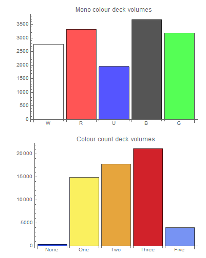
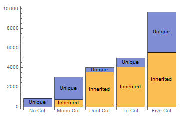
This shows some disparity in colour popularity. A deck with just blue cards being nearly half as frequent as one with just black. More stark is the massive preference of one, two, and three colour decks over the restrictive colourless and permissive five colour decks. We can also measure the variety of cards available to these decks (averages across colour count, code lost).

- Card popularity -

Presume that cards have clear variations in quality. This should affect occurrence frequency, we expect a good card to be chosen over a bad one. Does the data reflect this?

totalCardUse = Total[Total /@ denseFlagArrays];
ListLogPlot[
    Cases[Sort[totalCardUse], Except[0]]/Total[Length /@ denseFlagArrays], 
    Ticks -> {Automatic, {#, #, {1, 0}} & /@ (2^Range[-12, 0, 3])}]

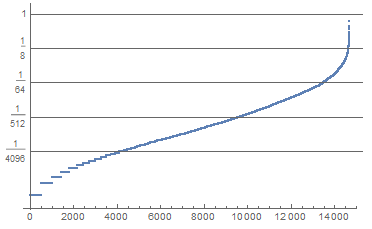
This log plot shows whilst most cards appear in a very small number of decks, a few cards appear a lot. Presumably these cards are 'good' cards. I explore the most frequent card.

totalCardFreq = totalCardUse/Total[Length /@ denseFlagArrays];
N[totalCardFreq[[Ordering[totalCardUse, -1][[1]]]]]
cardList[[18000 - Ordering[totalCardUse, -1][[1]]]][[1]]
cardList[[18000 - Ordering[totalCardUse, -1][[1]]]][[2, {4, 7}, 2]]

Used in a whopping two thirds of decks, the card 'Sol Ring' costs one mana point, and returns two mana points every turn. In absolute terms this info is meaningless, so I dig out cards with exactly the same effect for comparison.

atributeRef = Position[cardList[[;; , 2, ;; , 1]], "text", 2];
similarTextCards = 
    Pick[atributeRef[[;; , 1]], 
       StringMatchQ[cardList[[#[[1]], 2, #[[2]], 2]], 
         "{T}: Add {2} to your mana pool."] & /@ atributeRef];

cards = cardList[[similarTextCards[[#[[1]]]], 2, #[[2]], 2]] & /@ 
    Position[cardList[[similarTextCards, 2, ;; , 1]], "cmc", 2];
freqs = N[totalCardFreq[[18000 - similarTextCards]]];
order = Ordering[cards];

cards[[order]]
freqs[[order]]

There are five other cards bearing this text, the cheapest costing 3 times as much, and seen thirty times less often. Given the specificity of the text one may assume this type of effect is seen on a lot of cards, but that Sol Ring is disproportionately low cost.

Measuring card interaction

There are various challenges in trying to establish card distance. An immediate guess is co-occurrence, does card A appear with card B more than is probable? However due to the 100 card restriction, a pair of functionally identical cards that fill an important strategic role in a deck may be chosen one at a time. If this is the case then a direct co-occurrence measurement will miss extremely similar cards.

To combat this I tried to investigate the probability influence held by individual cards.

Taking a single source card, we average the deck lists it's found in to get the probabilities that each other card shares a deck with the source card. We then average the decks these cards are found in. This second set of card probabilities reflects the average makeup of decks similar to the source deck. By dividing the first average by the second, we measure the difference between the broader composition and the specific compositions including our source card. The discrepancies approximate the influence of the source card on selection of other cards.

This yields a good pairwise influence between cards. It isn't the similarity metric I was digging for, but it is very interesting.

First the small colourless deck set is reduced to its most frequent cards (removing the noise dominated low volume discrete sampling)

cardUseTotals = Total /@ # & /@ lightFlagRefArrays;
odds = N[cardUseTotals[[1]]/Dimensions[lightFlagRefArrays[[1]]][[2]]];

frequentQ = # >= 0.05 & /@ odds;
frequentRefs = Position[frequentQ, True][[;; , 1]];

The procedure described above is implemented, and pruned down to the frequent set.

cardDecks[col_, ref_] := ArrayRules[lightFlagRefArrays[[col, ref]]][[;; -2, 1, 1]];
usedDeckCardTally[col_, ref_] := Total[lightFlagArrays[[col, cardDecks[col, ref]]]];

coocuranceActual = (usedDeckCardTally[1, #] & /@ Range[Length[odds]]) (1 - IdentityMatrix[Length[odds]]);
coocuranceOdds = (coocuranceActual/Total[coocuranceActual]);
deviations = Quiet[coocuranceOdds[[#]] / Total[N[coocuranceOdds[[#]] coocuranceOdds]]] & /@ frequentRefs;
frequentDeviations = deviations[[;; , frequentRefs]];

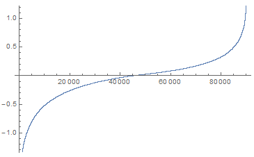
A quick sanity check hoping that positive and negative influences balances each other out looks promising.

ListPlot[Sort[Log[Flatten[frequentDeviations]]]]

The influences can then be ranked to sample the strongest positive card interactions.

order = Ordering[Flatten[frequentDeviations]];
order2D = Select[
  QuotientRemainder[# - 1, Length[frequentDeviations]] + {1, 1} & /@ Reverse[order], 
    And[#[[1]] != #[[2]], requentDeviations[[#[[1]], #[[2]]]] > 0.] &][[;; ;; 2]];

cardData[col_, ref_] := cardList[[18000 - colourCardSets[[col, ref]]]]
Log[frequentDeviations[[#[[1]], #[[2]]]]] & /@ order2D[[;; 10]]
cardData[1, frequentRefs[[#]]][[;; , 1]] & /@ order2D[[;; 10]]

These associations are immediately promising, the names alone hint at synergy!

I'll betray Wolfram tradition here by omitting the CommunityGraphPlot generated by these adjacencies. I'm still muddling through the probabilities and relationships required to find a decent similarity or global quality metric in this data.

All input very welcome.

David

Attachments: